


Rod-like colloidal particles are known to display an isotropic-nematic phase transition on increase of concentration, as predicted already by Onsager. Both natural clay particles and synthetic rods tend to be polydisperse, however, and the question arises how to allow for this in comparing experimental observations with theory. Experimental data for a wide range of samples (both from the literature and the new results) have been collated, with aspect ratios ranging from 14 to 35. As a characteristic, the concentration is taken where half of the sample volume is nematic. Experimental data agree well with predictions for monodisperse finite aspect ratio rods. However, compared to these predictions, the width of the transition (taken as the ratio of isotropic and nematic limiting concentrations) is noticeably broadened. Still, in most cases, the transition can be characterised by a linear increase of the nematic phase volume with sample concentration. The transition width is in broad agreement with theoretical predictions for infinitely thin rods.
I. INTRODUCTION
Suspensions of rod-like colloidal particles are of interest as they have been shown to be effective rheology modifiers in formulations.1 It has also been seen that the addition of the colloidal rods to plastics can greatly enhance the properties of the material.2 Interest in the behaviour of these particles has also been strong in the liquid crystal community since Zocher and Langmuir made initial studies describing in detail the phase separation observed in colloidal samples of V2O53 rods and bentonite plates,4 respectively. Many non-spherical (rod-like or disk-like) colloids have since been shown to reproducibly form a nematic phase.5,6 To describe the spontaneous alignment of colloidal particles into a nematic phase, Onsager developed a theory for non-interacting (or “hard”), infinitely thin, monodisperse rods.7
Few experimental model systems are monodisperse, and in practice, particles are never infinitely thin. The phase behaviour of hard spherocylinders with aspect ratio up to 60 was determined using computer simulations by Bolhuis and Frenkel8 and by McGrother for aspect ratios below 5.9 It was shown that on increasing the number density of monodisperse, hard particles in a sample, four phases can be found in turn: isotropic, nematic, smectic, and crystal (a columnar phase also observed by Bolhuis appeared metastable with respect to the crystal phase). It was also reported that the nematic and smectic phases are absent from the phase diagram of rods with an aspect ratio <3.7. The number density of the particles needed to observe these phase transitions is highly dependent on the aspect ratio.
The polydispersity of the system also has a large effect on the phase behaviour. Bates showed that polydispersity of hard spherocylinders would inhibit the smectic phase from forming.10 The effect of polydispersity on the isotropic-nematic (IN) transition was investigated by Lekkerkerker et al. for bidisperse, infinitely thin rods. They showed that the coexistence region broadens on increase of the polydispersity.11 These predictions could provide a good explanation for the experimental observations by Buining et al. on suspensions of (synthetic) boehmite rods.12 The phase behaviour of rod-like particles with continuous size distributions was studied by Speranza and Sollich13 and Wensink and Vroege.14 The formation of two nematic phases has also been observed in cases of high polydispersity both experimentally12,15,16 and in theory.17
Some semi-flexible polymers also form a nematic phase and these samples can also have a noticeable polydispersity in their lengths and so the aspect ratio. Ghosh and Muthukumar built on work by Warren18 and Sollich and Cates19 who explored the thermodynamics of polydisperse phase behaviour by calculating the cloud and shadow curves for the isotropic-nematic transition for semi-flexible rods.20
Sepiolite has previously been used as a source of rod-like colloidal particles.15 It has a crystal structure of alternating mineral and zeolitic channels running along the particle length. Zhang found that sepiolite particles, dispersed in non-aqueous solvent using an adsorbed steric stabiliser, phase separate and display a nematic phase.15 Yasarawan took advantage of the zeolitic channels in sepiolite by replacing the zeolitic water molecules with dye molecules to indicate concentration and orientation of the particles in situ.21
The source mineral particles are quite polydisperse. Particles of a limited degree of polydispersity can be obtained by fractionating, as was done in Refs. 15 and 21; however, this comes at the expense of yield. Here, we explore variations on the original recipe, paying attention to the yield as well as the properties of the resulting samples. Together with previously published data, aspect ratios ranging from 14 to 35 are covered and varying degrees of polydispersity. We show that the location of the IN transition compares quite well with predictions based on monodisperse rods; the width of the transition is compared with predictions for infinitely thin particles. This may serve as a practical guide on where to expect such “hard particle” dispersions to display an IN transition. Through better understanding of the conditions needed for nematic phase formation, it would greatly aid industrial and commercial purposes as the rheology and properties of a dispersion will be noticeably different when in a nematic phase.
II. EXPERIMENTAL
The sample preparation was adapted from the procedure used by Zhang and van Duijneveldt.15 The sepiolite clay used was B20 grade from Tolsa, in which the bare clay is already treated with an (undisclosed) surfactant, believed to be a quaternary amine. A 100 ml suspension of 5 wt. % B20 sepiolite in dried toluene was made and put under high shear for 5 min at 24 000 rpm (Ultra Turrax basic T-18, S18-10G blade), shaken by hand to break down any gel structure formed, and high shear mixed for a further minute. To this, a 20 wt. % solution of SAP-230TP (modified poly(isobutene),22 Infineum) in dried toluene was added so that there was a 2:1 weight ratio of sepiolite to SAP. The sample was shaken by hand for a minute, resulting in a noticeable drop in viscosity. The sample was then centrifuged at 3000 × g for 30 min (Sorvall Legend T, 6 × 94 ml fixed angle rotor) to remove any large clusters and then the supernatant was centrifuged at 11 000 × g for 1 h to remove the excess stabiliser, with the sediment being redispersed in dried toluene to make a stock sample of roughly 20 wt. %. Exact wt. % and yields were calculated by drying a small sample and C, N, and H elemental analysis (Eurovector EA3000) was used to find the organic fraction of the solids to calculate the bare clay mass of the dried sample. The core volume fraction of the clay particles then follows from Eq. (1), where ρsep = 2.10 g/cm3,23 the solvent density ρtol = 0.87 g/cm3, and wc is the dry mass fraction of the sample multiplied by fm, the weight fraction of the dried sample which is mineral and not the organic stabiliser. Note that implicitly, the density of the organic stabiliser is taken to be equal to that of the solvent,22
For phase behaviour observations, the stock sample was diluted to 2 different concentrations and the nematic phase content was observed in a home made light box through crossed polarising filters (200 × 200 mm, <0.004 transmission crossed, Edmund Optics) and backlit using a fluorescent light panel (MedaLight LP-20). Images were taken using a camera (Nikon D40, 18-50 mm Nikon lens) to make measurements of the nematic volume fraction. To get the particle dimensions, transmission electron microscopy (TEM; JEOL JEM 1200 EX) was done on a 0.01 wt. % sample dried on to a carbon coated copper grid (200 mesh × 125 μm pitch, Sigma) and by counting 200 rods for the length and 60 for the diameter, using separate magnification images to determine lengths and diameters (Figure 1).
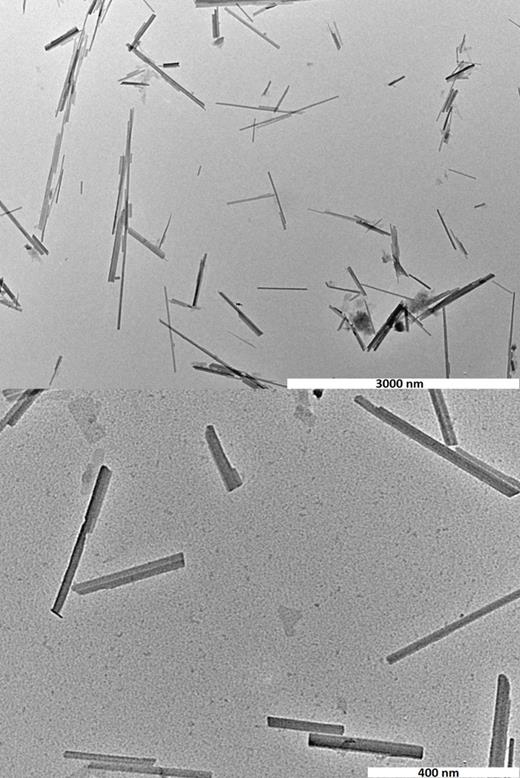
Example of TEM images used to size particles from sample 5, with the top images used for length (scale bar—3000 nm) and the bottom image used for diameter (scale bar—400 nm).
Example of TEM images used to size particles from sample 5, with the top images used for length (scale bar—3000 nm) and the bottom image used for diameter (scale bar—400 nm).
The standard procedure outlined above was used to prepare sample 1 before trialling variations as follows. Sample 2 was prepared with the shearing carried out after the addition of the SAP stabiliser, to test whether the addition of SAP before dispersion would crosslink the particles into clusters requiring a much higher energy to break up. Sample 3 was made by stirring the SAP stabiliser in excess for 24 h before the centrifugation process to examine whether this would result in a better stabilisation. Sample 4 was prepared using an ultrasonic bath (IND 500D, Ultrawave) for 5 min before the high shear treatment, as it has previously been reported that high levels of sonication can produce shorter rods.24 Sample 5 had a 2.5 wt. % starting sepiolite concentration with the SAP stabiliser being added in the same ratio as before as the lower concentration would affect the sedimentation of the particles during the fractionation process. Sample 6 had only half the amount of SAP added and finally, sample 7 was prepared using a lower shear of only 4000 rpm on the Ultra Turrax to determine if a stable dispersion could be made without the gelation seen from the high shear stage. The fractionation and analysis of these samples were kept consistent so any changes in the results would be due to the dispersion process.
III. RESULTS AND DISCUSSION
The dimensions, yield, organic content, and phase behaviour of the samples are summarised in Table I. The table shows the core mineral length (L) and diameter (D) and their standard deviation σ from the TEM data. The first group of data in the table used sepiolite S9 particles (bare particles), the second group of data was for B20 grade (organically modified) sepiolite, and finally the last group of data was for synthetic boehmite particles, treated with the same SAP stabiliser12,25 where core volume fractions for Ref. 12 were re-calculated following Ref. 25.
Summary of rod-like particle samples. All dimensions are in nm for the core particles without stabiliser.
| Mineral | Yield (%) | 〈L〉 (σL) | 〈D〉 (σD) | Organic (wt. %) | ϕI core | ϕN core | |
|---|---|---|---|---|---|---|---|
| Reference 26 | S9 | … | 852 (±344) | 18a (±4.0) | 16 | 0.010 | 0.085 |
| Reference 26 | S9 | … | 652 (±264) | 18a (±5.0) | 16 | 0.018 | 0.101 |
| Reference 26 | S9 | … | 332 (±126) | 18a (±4.5) | 16 | 0.025 | 0.154 |
| Reference 15 | B20 | … | 924 (±360) | 27 (±4.0) | 20 | 0.047 | 0.126 |
| Reference 15 | B20 | … | 1182 (±343) | 27 (±4.0) | 20 | 0.037 | 0.094 |
| Reference 15 | B20 | … | 577 (±127) | 26 (±4.0) | 20 | 0.062 | 0.149 |
| 1 | B20 | 65 | 843 (±412) | 31 (±17) | 23 | 0.011 | 0.121 |
| 2 | B20 | 66 | 884 (±563) | 30 (±12) | 22 | 0.009 | 0.125 |
| 3 | B20 | 66 | 944 (±588) | 32 (±13) | 26 | 0.018 | 0.125 |
| 4 | B20 | 59 | 1070 (±669) | 29 (±11) | 24 | 0.014 | 0.102 |
| 5 | B20 | 65 | 906 (±558) | 25 (±9.0) | 24 | 0.008 | 0.114 |
| 6 | B20 | 63 | 925 (±501) | 27 (±12) | 22 | 0.025 | 0.198 |
| 7 | B20 | 23 | 954 (±588) | 30 (±15) | 25 | 0.015 | 0.067 |
| Reference 12 | Boehmite | … | 200 (±104) | 10 (±4.5) | 16 | … | … |
| Reference 25 | Boehmite | … | 250 (±63) | 9.4 (±2.4) | 20 | … | … |
The value is not taken from the TEM data but from a subsequent analysis of barometric height distribution in rod-sphere mixtures reported in Ref. 26.
For the dimensions marked with a superscript “a,” the value is not taken from the TEM data but from a subsequent analysis of barometric height distribution in rod-sphere mixtures reported in Ref. 26. The yield is expressed as the non-organic solids in the final suspension as a percentage of the initial start mass of sepiolite in the preparation.
The particle number density is calculated as ρ = ϕcore/v0 with v0 = LD2 the volume of one particle (both sepiolite and boehmite are considered to be well represented by a cuboidal shape).15,25 The TEM is able to detect the dimensions of the core particles but when in suspension the steric stabiliser extends into solution. The effective layer thickness is taken to be δ = 4 nm.27 Fig. 1 shows a few bundles of particles which were believed to form in the drying process and the diameter of individual particles was sized. Effective particle dimensions are therefore calculated as D∗ = D + 2δ and L∗ = L + 2δ. Henceforth, comparisons will be made with predictions for hard spherocylinders of dimensions L∗ and D∗ (one could argue for a somewhat different definition of effective diameter, to allow for the difference in particle shapes,26 but this has not been done here).
As this paper focuses on the role of polydispersity, it is appropriate to take this into account explicitly in any calculations. Leaving this correction out would lead to a worse agreement between experiment and simulations in Fig. 2. Phillips found that the length and diameter of the sepiolite rods are independent of each other.24 The effective average aspect ratio can therefore be calculated (Eq. (2)) using a Taylor expansion truncated at second order.28 The polydispersity correction amounts to at most 25% and it is not likely that higher order terms would resolve the differences between theory and experiment seen below,
In order to calculate 〈D∗/L∗〉, an equivalent expression is used with D∗ and L∗ interchanged.

In most cases, it is found that there is a linear dependence between the volume fraction of the clay and the volume of nematic phase in the sample.15 Therefore, linear fits of the nematic volume fraction as a function of sample concentration were used to obtain the core volume fractions corresponding to nematic fractions of 0 and 1, ϕIcore and ϕNcore, respectively. Results are included in Table I. For the samples of boehmite,12,25 a non-linear relationship between the volume fraction and nematic fraction was reported. For these samples, the literature values have been used.
In presenting the phase behaviour of hard spherocylinders, Bolhuis and Frenkel use a scaled density variable c which already factors out the main dependence of aspect ratio.8 Here, c is calculated using the effective particle dimensions as
Combining this expression with the preceding definitions allows calculating c starting from ϕcore as
where once more the polydispersity in diameter has been included in evaluating an average value. In order to compare with simulation data, c50 is used, representing a sample with a nematic fraction of 50%. Further details on data analysis and error bars are given in the supplementary material.29
In previous studies, the yield was not quoted, but for the present work (Table I) the various preparation routes all produce similar results, apart from sample 7 which was subject to a reduced level of shear. This shows that high shear is indeed required in order to break up aggregates in the suspension process.
By comparing the dimensions of the sepiolite particles, it is clear that there is a difference between the B20 grade of clay used in this report as well as by Zhang and the S9 grade used by Yasarawan. The average dimensions of the samples made for this report were very similar to those seen by Zhang in the initial sample but it is clear that there is a lower level of polydispersity in the dispersion made by Zhang and Yasarawan; note that they used an additional fractionation step in purifying the rods. It is also worth noting that the batch of B20 clay was not the same as that used previously and so slight variations in polydispersity could have arisen through raw material differences.
The location of the IN transition, expressed as c50, is shown in Fig. 2 as a function of 〈D∗/L∗〉. Across a wide range of aspect ratios (14 to 35), the experimental data are quite close to the computer predictions for hard spherocylinders by Bolhuis and Frenkel.8 The notable exception is Sample 7 which has a rather low c50 value, possibly as a results of aggregates remaining in this sample.
Compared to the predictions for monodisperse rods, all experimental phase diagrams show a much wider coexistence region between the isotropic and nematic phases. Polydispersity in aspect ratio is likely to be an important factor in this. In Fig. 3, the width of the transition (expressed as ϕI/ϕN) is therefore plotted against the relative standard deviation (RSD) of the aspect ratio (σL∗/D∗/〈L∗/D∗〉). The figure compares all data, covering a range of values for the aspect ratio.

The width of the coexistence region, expressed as ϕI/ϕN, as a function of the relative standard deviation in aspect ratio. The crosses are data points from Lekkerkerker et al.11 with the solid line as a linear fit; data from Wensink and Vroege14 for a Schulz distribution (closed stars) and log-normal distribution (open stars) joined by lines to guide the eye. The other symbols are as in Fig. 2.
The width of the coexistence region, expressed as ϕI/ϕN, as a function of the relative standard deviation in aspect ratio. The crosses are data points from Lekkerkerker et al.11 with the solid line as a linear fit; data from Wensink and Vroege14 for a Schulz distribution (closed stars) and log-normal distribution (open stars) joined by lines to guide the eye. The other symbols are as in Fig. 2.
Predictions for bidisperse systems of infinitely thin rods11 are included in Fig. 3 for comparison. Even for such a simple model, the detailed phase behaviour is remarkably complex; specific predictions for binary mixtures of equal numbers of short and long rods were taken in order to arrive at the data points represented by crosses in the figure. Plotted in this way, a linear trend emerges for the predicted width of the transition as a function of RSD. Note it would also be possible to choose skewed bimodel distributions but that has not been pursued here.
The rod lengths and diameters are typically well described by log-normal distributions.15 In order to achieve good accuracy, different magnification TEM micrographs were used to characterise L and D so direct experimental data for the distribution of L/D is not available.21 However, there is evidence that the two distributions are independent24 and therefore it may well be appropriate to describe (L/D) with a log-normal distribution as well. The phase behaviour of rod-like particles with continuous aspect ratio distributions was considered by Speranza and Sollich13 and Wensink and Vroege.14 The latter paper includes cloud curves both for the isotropic and nematic phases which allow a direct comparison with the data in Figure 3. Predictions have been included for both a Schulz distribution of aspect ratios and a log-normal distribution. For the latter, it was necessary to truncate the aspect ratio in order to make the problem well-defined and the prediction shown in Figure 3 is for aspect ratios truncated at a value of 10 times the average.
The theoretical predictions fall slightly below the values taken from Lekkerkerker et al.11 This is already visible for the monodisperse case (RSD = 0) and may in large part be due to the different trial functions used in the theoretical approaches.30 The theoretical curves extend to RSD values up to about 0.4 and are fairly close to the available experimental data (all from previous studies). The new experimental data presented in this paper relates to even more polydisperse samples, with RSD values around 0.6. These data are consistent with a continuing downward trend in ϕI/ϕN as RSD increases, as is also indicated by the bimodal theory.
A key premise of these calculations is that the particles are considered to have steeply repulsive (hard) interactions. It is possible that in some cases residual particle attractions remain, as a result of incomplete steric stabilisation.31 Previous computer simulations32 and experiments33 for rod—polymer mixtures (displaying depletion attractions between rods) show that, upon introducing particle attractions, the location of the phase transition is initially not affected, but the phase coexistence widens. This may apply to some of the samples with particularly wide coexistence regions.
IV. CONCLUSIONS
This work has shown that when dispersing sepiolite to form non-aqueous suspensions, the processing of the particles has little effect on the yield, dimensions, and phase behaviour of the particles. An effective method for fractionating samples has been demonstrated by Donkai34 and Zhang,15 based on the isotropic-nematic phase transition itself—the resulting daughter phases are more monodisperse and of different aspect ratios. Inevitably, however, this implies a reduction in yield for a specific fraction.
By combining the data obtained here with previous results on sepiolite as well as boehmite suspensions, it has been shown that the location of the IN transition can be predicted well by theory for monodisperse hard spherocylinder suspensions of an aspect ratio corresponding to the sample average.
The width of the transition in some cases approaches that predicted for infinitely thin, bidisperse rod mixtures; in other cases, however, the predictions made for a continuous skewed distribution fit the experimental data better. Taken together, these results provide useful guidance on the concentrations where one could expect suspensions of well-stabilised, rod-like particle suspensions to undergo an IN transition.
Acknowledgments
One of us (P.W.) was supported by a Ph.D. studentship (EPSRC, No. EP/J500379/1). We acknowledge Mr. J. Jones (Electron and Scanning Probe Microscopy Facility) for training and access to the electron microscope and Mr. D. Davis for carrying out the elemental analysis measurements. The sepiolite was a gift from Dr. M. Perez (Tolsa) and the SAP-230TP stabiliser was a gift from Dr. P. J. Dowding (Infineum).

