


1. Introduction
Although the two European national varieties of Dutch, viz. Belgian Dutch (BD) and Netherlandic Dutch (ND),Footnote a are highly related and mutually perfectly intelligible, they are characterized by an “uncommonly complex synchronic and diachronic relationship” (Grondelaers and van Hout Reference Grondelaers and van Hout2011, p. 199), which is embodied in increasingly diverging evolutions on various linguistic levels. While analysis of news bulletins, on the one hand, has manifested phonetic divergence since the 1930s (Van de Velde Reference Van de Velde1996), a study of naming preferences in two lexical fields, on the other hand, revealed a converging trend between 1950 and 1990 (Geeraerts, Grondelaers, and Speelman Reference Geeraerts, Grondelaers and Speelman1999), which, moreover, appears to have stagnated in the first decade of the current century according to a recent replication study (Daems, Heylen, and Geeraerts Reference Daems, Heylen and Geeraerts2015).
With regard to syntax, however, the exact relationship between BD and ND is less clear. The main reason for this is the virtually undisputed idea among laymen and analysts that BD and ND are different surface manifestations of an identical “syntactic motor” (e.g. Van Haver Reference Van Haver1989, p. 41; Taeldeman Reference Taeldeman1992, p. 47), and little is known about syntactic differences which are not categorical or heavily mediatized (cf. Rohdenburg and Schlüter Reference Rohdenburg and Schlüter2009, pp. 1–2 for similar observations regarding grammatical differences between British and American English). As a consequence of this ideological bias, and the absence of large-scale corpora and affordable statistical tools before the 2000s (cf. Grondelaers and van Hout Reference Grondelaers and van Hout2011, p. 200), only a limited number of syntactic variables has hitherto been shown to be sensitive to national constraints. Among the regression-based studies which have since then become available, it is striking to notice that Dutch researchers almost completely ignore the national factor in their models (e.g. van Bergen and de Swart Reference van Bergen and de Swart2010 on scrambling; van de Velde, Kempen, and Harbusch Reference van de Velde, Kempen and Harbusch2015 on lexical biases in Dutch dative structures in VO and OV clauses; Vogels and van Bergen Reference Vogels and van Bergen2017 on the syntactic position of low-accessible subjects), whereas Belgian researchers (e.g. Grondelaers, Speelman, and Geeraerts Reference Grondelaers, Speelman, Geeraerts, Morin and Sébillot2002b, Reference Grondelaers, Speelman, Geeraerts, Kristiansen and Dirven2008 on existential er; Speelman and Geeraerts Reference Speelman and Geeraerts2009 on causative constructions with the auxiliaries doen “do” and laten “let”) did not only find quantitative (i.e. proportional), but also qualitative differences between the national varieties, to the extent that constructional preferences in ND appeared to be determined by fewer and more robust predictors than in BD. Grondelaers et al. (Reference Grondelaers, Speelman, Geeraerts, Kristiansen and Dirven2008) proposed that the structural differences between the BD and ND distribution of existential er reflect crucial differences in the “syntactic motor” of these varieties: regression analysis showed that constructional preferences in BD were determined by a “case-based” consideration of various higher-level syntactic, semantic, and pragmatic features, whereas the more predictable ND appeared to rely to a higher extent on collocations between specific lexemes and er (see Section 2).
The present article aims to address the structural differences between the European national varieties of Dutch by revisiting the post-verbal distribution of er “there” in adjunct-initial existential constructions, and extending the chain of empirical analyses to include bare lexical information. If er’s ND distribution is to a large extent lexically determined, it could be hypothesized that a “lazy” learning algorithm such as memory-based learning (MBL) (Daelemans and van den Bosch Reference Daelemans and van den Bosch2005), which builds on similarity to specific examples in memory to solve a classification problem (see Section 3), should be able to predict constructional choices to a considerable extent on the basis of no more than raw lexical input. For BD, in which the distribution of er is to a higher extent dependent on higher-level processing factors related to the contextual probability of the upcoming subject (see Section 2), we assume that raw lexical input does not suffice, and that syntactically more informed or other higher-level predictors are needed in order to reach a comparable classificatory accuracy.
The remainder of the article is structured as follows. Section 2 presents some groundwork on existential er, summarizing what is known from previous corpus-based and experimental research. Section 3 introduces MBL. Data extraction and feature selection are covered in Section 4. Section 5 details the experimental setup and presents and discusses the results. In Section 6, we take a closer look at the errors made by the classifier. Finally, Section 7 theorizes some of the conclusions.
2. National variation in the distribution of existential er “there”
Among syntacticians, the post-verbal distribution of existential or presentative er “there” is known as one of the most notoriously complex phenomena in Dutch grammar (see e.g. van der Wouden Reference van der Wouden2009). Its characterization in the 1997 edition of the Algemene Nederlandse Spraakkunst (ANS) —the Dutch reference grammar—testifies to this complexity:
For the distribution of presentative er, no strict rules can be given: it may be optional, there may be semantic or stylistic differences involved, and there is especially a lot of individual, sometimes also regional, variation in its use. (Haeseryn et al. Reference Haeseryn, Romijn, Geerts, de Rooij and van den Toorn1997, p. 473, translation ours)Footnote b
Rather than trying to account for the distribution of er, the authors cite almost every conceivable source of variation, which is hardly helpful.
The following examples illustrate the standard sentence-initial use of er in (1a), which is comparable to the use of existential there in English, whereas (1b) and (1c) illustrate the adjunct-initial existential construction, in which the locative adjunct constituent in haar brooddoos “in her lunchbox” is fronted, and er may either or not occur post-verbally.
-
(1) a. Er zat een broodje in haar brooddoos.
there sat a sandwich in her lunchbox
‘There was a sandwich in her lunchbox.’
-
b. In haar brooddoos zat (er) een broodje.
in her lunchbox sat (there) a sandwich
‘In her lunchbox (there) was a sandwich.’
-
c. In haar brooddoos zat (er) een worm.
in her lunchbox sat (there) a worm
‘In her lunchbox (there) was a worm.’
In a series of regression analyses, Grondelaers et al. (Reference Grondelaers, Speelman, Geeraerts, Morin and Sébillot2002b, Reference Grondelaers, Speelman, Geeraerts, Kristiansen and Dirven2008) found that post-verbal er’s distribution is not unpredictable but motored by a number of higher-level features which are parameters of er’s processing function, viz. signaling an upcoming low probability subject, such as een worm “a worm” in (1c) above (see especially Grondelaers et al. Reference Grondelaers, Brysbaert, Speelman and Geeraerts2002a and Reference Grondelaers, Speelman, Drieghe, Brysbaert and Geeraerts2009 for experimental evidence to this effect). Factors identified as predictors of er are all determinants of the subject’s contextual probability: sentence-initial locative adjuncts, and especially concrete locative adjuncts, severely reduce the set of potential subjects (e.g. in haar brooddoos “in her lunchbox” constrains the subject to dry lunch food), and so do specific verbs. Together with the external factors region (the higher Belgian preference for er) and register (the higher frequency of er in less edited or more informal genres), the internal factors adjunct concreteness and verbal specificity suffice to predict the distribution of er quite well.Footnote c It will be noticed that this high predictability contrasts sharply with the “no strict rules” pessimism in the ANS quoted above.
Crucially, Grondelaers and colleagues found substantial quantitative and qualitative differences between separate regression models for BD and ND. For ND, a high classificatory accuracy was obtained on the basis of the predictors adjunct concreteness and verbal specificity, and the register factor played no role whatsoever; BD required inclusion of the register factor as well as additional higher-order parameters of the predictability of the upcoming subject to obtain a reasonable fit, which was never, however, as high as in ND (Grondelaers et al. Reference Grondelaers, Speelman, Geeraerts, Kristiansen and Dirven2008).
Grondelaers et al. (Reference Grondelaers, Speelman, Geeraerts, Kristiansen and Dirven2008) accounted for this crucial national divergence in terms of an evolutionary difference, and more particularly the fact that standard language in the Netherlands is older and more entrenched than in Belgium (for detailed descriptions of the standardization processes in the Netherlands and Belgium—and especially the delayed standardization of BD—see, among many others, Geeraerts et al. Reference Geeraerts, Grondelaers and Speelman1999, pp. 13–8; Marynissen and Janssens Reference Marynissen and Janssens2013, pp. 88–98; Willemyns Reference Willemyns2013). Two effects of this advanced evolution of ND are (i) a functional specialization, whereby the adjunct-initial template in (1b)–(1c) is typically reserved for discourse-contextually predictable subjects, while unpredictable subjects are restricted to the related er-initial template in (1a); and (ii) lexical specialization, the fact that er does not only co-occur with a limited number of constituents in ND (notably with concrete adjuncts and specific verbs), but also with a (more) restricted set of specific lexemes (Grondelaers et al. Reference Grondelaers, Speelman, Geeraerts, Kristiansen and Dirven2008, pp. 194–196).
Especially the latter effect—the impact of raw lexemes on the distribution of er—cannot straightforwardly be tested in regression analysis, the de facto standard analytical tool in corpus-based studies of syntactic variation (Gries Reference Gries2017). This has been noted before in research focusing on syntactic variation which is lexically co-determined. In a study of the so-called dative alternation (the choice between The evil queen gave Snow White the poisonous apple and The evil queen gave the poisonous apple to Snow White), Theijssen et al. (Reference Theijssen, ten Bosch, Boves, Cranen and van Halteren2013) compared traditional regression modeling, which builds on researcher-defined higher-level features, with MBL, a machine learning algorithm which classifies unseen data by extrapolating from specific instances in memory without abstracting away from the actual data (Daelemans and van den Bosch Reference Daelemans and van den Bosch2005; cf. Section 3 infra). Crucially, Theijssen et al. (Reference Theijssen, ten Bosch, Boves, Cranen and van Halteren2013) found that MBL easily rivaled the performance of traditional regression analyses, which led them to call into question the need for researcher-defined higher-level features in the modeling of syntactic alternations. A theoretical advantage of the fact that MBL does not rely on higher-level features is that it does not make any claims about the way in which abstractions are shaped, nor does it make a priori distinctions between “regular” and “irregular” instances (van den Bosch and Daelemans Reference van den Bosch and Daelemans2013). Therefore, MBL has by some authors been claimed to be a cognitively more plausible modeling technique than regression models (Theijssen et al. Reference Theijssen, ten Bosch, Boves, Cranen and van Halteren2013; Milin et al. Reference Milin, Divjak, Dimitrijević and Baayen2016).
In view of all the foregoing, three research question (RQs) will be addressed in this article:
-
RQ1 Can a learning algorithm such as MBL learn the distribution of er in BD and ND on the basis of raw lexical input—and lexical input only—or does the classifier need linguistically enriched information?
-
RQ2 Does the alleged lexical specialization of er in ND materialize in comparatively higher predictive success on the basis of raw lexical input than in BD? And, conversely, does the MBL analysis of er’s BD distribution require linguistic enrichment?
-
RQ3 Does the lexical specialization which is hypothesized to streamline er-production in ND entail that the more “noisy” BD data are less suited to learn er’s ND distribution? And, conversely, can a Belgian classifier learn er-preferences from the more “lexically entrenched” ND material?
3. Memory-based learning
MBL is a machine learning method that builds on the combination of two powerful mechanisms: storing some representation of the data in memory, and inducing the solution to a classification problem from previous experiences through analogical reasoning over the most similar cases in memory (Daelemans and van den Bosch Reference Daelemans and van den Bosch2005). Even though MBL does not abstract away from the individual instances in the training set, unlike for example regression analysis, it is still able to generalize to new, unseen instances. MBL builds on the assumption that “in learning a cognitive task from experience, people do not extract rules or other abstract representations from their experience, but reuse their memory of that experience directly” (Daelemans and van den Bosch Reference Daelemans and van den Bosch2005, p. 5). As such, MBL could be considered an implementation of so-called usage-based theories of language, which assume that linguistic knowledge—the system, or “competence”—is shaped (and continuously re-shaped) through individual experience with language, and as such cannot be separated from actual language use or “performance.” As a consequence, individual utterances have a direct impact on cognitive representations of linguistic knowledge (cf. e.g. Bybee Reference Bybee2006, Reference Bybee2010).
We used the MBL implementation in the software package TiMBL (Tilburg Memory-Based Learner; Daelemans, Zavrel, and van der Sloot Reference Daelemans, Zavrel and van der Sloot2018). To illustrate how TiMBL operates, Daelemans and van den Bosch (Reference Daelemans and van den Bosch2005, pp. 7–8) give the example of learning the past tense of English verbs, where “learning” is conceived of as a mapping from an input—the infinitive of a verb—to an output—the preterite of that verb (e.g. work
 $\rightarrow$
work-ed
, sing
$\rightarrow$
work-ed
, sing
 $\rightarrow$
sang). In order for TiMBL to make sense of the input, it has to be transformed into a fixed feature vector, with, for example, information on the syllable structure of the infinitive. This is done for every verb in a training set. When encountering a new verb, the classifier compares that verb’s syllable structure to the syllable structures of the k-nearest neighbors in memory, with proximity in memory being defined as having a similar feature vector. Translating this to Dutch existential constructions: in order to learn the distribution of er in new instances of the construction, the classifier scans its memory to find the k-nearest neighbors of the instance to be classified and then extrapolates the probability of er from these nearest neighbors; the classifier then decides whether or not er is to be inserted in the instance at hand.
$\rightarrow$
sang). In order for TiMBL to make sense of the input, it has to be transformed into a fixed feature vector, with, for example, information on the syllable structure of the infinitive. This is done for every verb in a training set. When encountering a new verb, the classifier compares that verb’s syllable structure to the syllable structures of the k-nearest neighbors in memory, with proximity in memory being defined as having a similar feature vector. Translating this to Dutch existential constructions: in order to learn the distribution of er in new instances of the construction, the classifier scans its memory to find the k-nearest neighbors of the instance to be classified and then extrapolates the probability of er from these nearest neighbors; the classifier then decides whether or not er is to be inserted in the instance at hand.
Which specific instances are taken into account as nearest neighbors—and by consequence the predictive success of the classifier—depends on several hyperparameters. First one is the similarity metric (m), which computes the distance between the test instance at hand and all instances in the training set, by comparing their respective feature vectors. In its most basic implementation, all features contribute equally, but features can also be weighted using some weighting metric (w), depending for example on prior (world) knowledge or hypotheses on their relative importance. A third parameter is the number of nearest neighbors considered for extrapolation (k). Finally, as an alternative to majority voting, in which each nearest neighbor has an equal vote, some form of distance weighting (d) can be employed, for instance by penalizing instances that are more dissimilar. Space limitations preclude a discussion of all possible hyperparameter values; for details, the reader is referred to Daelemans and van den Bosch (Reference Daelemans and van den Bosch2005, pp. 28–44).
4. Data
4.1 Data extraction
As indicated above, MBL needs labeled training data to be stored in memory, on the basis of which unlabeled test examples can be classified. We extracted the data from two large newspaper corpora. For the (ND) data, the 500-million-word Twente News Corpus (TwNC) was used (Ordelman et al. Reference Ordelman, de Jong, van Hessen and Hondorp2007), while for the BD data we used the highly comparable Leuven News Corpus (LeNC), which was compiled by the QLVL research group at the University of Leuven and currently contains 1.3 billion words. Both corpora are similar in design, consisting of materials from a collection of major Dutch and Flemish newspapers which have been published around the turn of the current millennium and are distributed and read nationwide.
The compilers of TwNC and LeNC have parsed all data with the Alpino parser, which is the current state-of-the-art dependency parser for Dutch (van Noord Reference van Noord2006). This allowed us to conveniently retrieve relevant instances of adjunct-initial existential sentences, which would be considerably harder using regular expressions on non-parsed text, as existential sentences are lexically highly, and in instances of the er-less variant even completely un(der)specified. Specifically, we extracted all sentences with the following syntactic structure:
-
(2) adjunct PP + main verb (+ er) + indefinite subject NP
In order to make extraction as efficient as possible in terms of precision and recall, we imposed a number of heuristic restrictions. For the indefinite subject, we limited ourselves to NPs with a nominal head node (thus excluding pronouns and proper names). Sentence-initial adjuncts were restricted to prepositional phrases (PP) with a nominal head node.Footnote d Next, since previous research had focused exclusively on variation in existential sentences with temporal and locative adjuncts (including their metaphorical uses, see Grondelaers et al. Reference Grondelaers, Speelman, Geeraerts, Kristiansen and Dirven2008, pp. 173–5), we limited the query to adjuncts which contain one of the prepositions the reference grammar ANS lists as typical or frequent prepositions in these types of adjuncts (cf. Haeseryn et al. Reference Haeseryn, Romijn, Geerts, de Rooij and van den Toorn1997, pp. 1194ff.). Finally, er itself could either or not occur between the main verb and the post-verbal subject.
For the present study, we exclusively extracted materials from the Dutch newspapers NRC Handelsblad (NRC) and Algemeen Dagblad (AD), and the Flemish newspapers De Standaard (DS) and Het Laatste Nieuws (HLN). In both countries, we selected newspapers along a formality dimension because this register variable was found to impact er-preferences in BD but not in ND (Grondelaers et al. Reference Grondelaers, Speelman, Geeraerts, Morin and Sébillot2002b; Reference Grondelaers, Speelman, Geeraerts, Kristiansen and Dirven2008; Reference Grondelaers, Speelman, Drieghe, Brysbaert and Geeraerts2009; and cf. supra): while many consider NRC and DS as “quality newspapers” that are geared toward an educated audience, AD and HLN are generally classified as “popular newspapers.” As could be expected from the separate regression analyses in Grondelaers et al. (Reference Grondelaers, Speelman, Geeraerts, Morin and Sébillot2002b, Reference Grondelaers, Speelman, Geeraerts, Kristiansen and Dirven2008), we found no statistically significant difference (at
 $\alpha=0.05$
) between er’s distribution in the ND quality and popular newspaper (
$\alpha=0.05$
) between er’s distribution in the ND quality and popular newspaper (
 $\chi^2_1=1.97$
,
$\chi^2_1=1.97$
,
 $p=0.16$
). For BD, for which there is much more data, the difference is statistically significant (
$p=0.16$
). For BD, for which there is much more data, the difference is statistically significant (
 $\chi^2_1=9.12$
,
$\chi^2_1=9.12$
,
 $p=0.003$
), but the effect size is very small (Cramér’s
$p=0.003$
), but the effect size is very small (Cramér’s
 $V=0.02$
; this is also apparent visually in Figure 1, in which the proportional difference between the latter two columns is very small). Given all this, we will proceed without taking the register dimension explicitly into account.
$V=0.02$
; this is also apparent visually in Figure 1, in which the proportional difference between the latter two columns is very small). Given all this, we will proceed without taking the register dimension explicitly into account.

Figure 1. Mosaic plot of er’s distribution across the four newspapers (NRC and AD for ND; DS and HLN for BD). The area of each tile of the plot is proportional to the number of observations it represents.
As can be appreciated in Figure 1, adjunct-initial existential constructions are much more frequent without (-ER) than with er (+ER) (an asymmetry that is well known, see Grondelaers et al. Reference Grondelaers, Speelman, Geeraerts, Morin and Sébillot2002b, Reference Grondelaers, Speelman, Geeraerts, Kristiansen and Dirven2008). However, this skewed distribution causes baseline accuracy for our models to be fairly high, especially in the TwNC data, which we remedied by downsampling the non-er cases, so that baseline accuracy for both the TwNC and LeNC data is set to 50%. For each national variety, from both newspapers, an approximately equal number of random instances were extracted and manually checked until we reached a total of 1000 instances; 500 with er and 500 without er.Footnote e
4.2 Feature selection
As one of the main goals of this article is to test the predictability of syntactic variation (within and across national varieties) on the basis of lexical input, we need a way to represent each corpus instance in a format that is interpretable for the TiMBL classifier, yet still meaningful in the light of our RQs. In view of RQ1—that is the question whether we can predict er-preferences on the basis of raw lexical material or whether some form of additional linguistic knowledge is needed—we created two types of datasets: one in which the features provided to the classifier consist of nothing more than the immediate lexical context, and one in which we used the Alpino dependency parses to extract from each instance those lexical features which have been shown in previous research to represent the key elements which determine er-choices. We will refer to the first type of instance representation as the window-based (WIN) approach, and to the second one as the parse-based (PAR) approach (cf. Pijpops Reference Pijpops2019, Chapter 7 for a similar procedure).
For the WIN approach, we identified for every instance in the balanced datasets the syntactic position (or “slot”) in which er occurs, or, in the instances where it is not realized, could have occurred. We subsequently extracted 5 items to the left and to the right of this position, which yielded 10 features in total. All words were converted to lowercase. In sentences with less than five words to the left or right of the er slot, an underscore was inserted as a padding character. Each feature in the dataset was separated by a white space, with the final feature being the class label, viz. +ER or -ER (cf. Daelemans et al. Reference Daelemans, Zavrel and van der Sloot2018, Chapter 4). Instances like (3)–(6) are thus represented as in Table 1 in the WIN format. The resulting datasets are henceforth referred to as LeNC-WIN and TwNC-WIN.
-
(3) In de Brusselse ziekenhuizen is er een schrijnend tekort aan vroedvrouwen.
in the Brussels hospitals is there a harrowing shortage of midwives
“In Brussels’s hospitals there is a harrowing shortage of midwives.”
(DS, 11 September 2003)
-
(4) In de badkuip stond geen water.
in the bathtub stood no water
“In the bathtub was no water.”
(HLN, 14 July 2000)
-
(5) Bij de fabriek in Amsterdam werken 285 werknemers.
at the factory in Amsterdam work 285 employees
“At the factory in Amsterdam work 285 employees.”
(NRC, 26 April 2004)
-
(6) Over twee jaar is er een WK.
in two years is there a World_Cup
“In two years there will be a World Cup.”
(AD, 26 June 2004)
Table 1. Slice of the WIN datasets (the first two examples are from LeNC and the last two are from TwNC)

L/Rn: nth word to the left/right of the er-slot.
Table 2 lists the number of distinct values (types) for each feature in LeNC-WIN and TwNC-WIN, as well as the number of types that occur in both datasets (overlap). This table shows that the overlap between the feature values in both varieties is generally rather sparse. The overlap is somewhat higher for features which tend to capture closed-class lexical items, such as prepositions and determiners, or several high- to mid-frequent verbs and nouns (e.g. the verb zijn “to be”; we will return to this in Section 6).
Table 2. Number of feature values in the WIN datasets

For the PAR approach, we employed a linguistically more informed way of feature selection. Although the WIN approach includes five words on either side of the item to be classified, it is uncertain that all the predictors known from previous research to be determinants of er’s distribution are actually included. This is the case in instances with long adjuncts, for example, like in (7), in which the temporal adjunct constituent op het moment dat De Visser en Rzasa hun gezicht lieten zien is 12 words long. In such cases, the nominal head of the adjunct, that is moment, falls out of the range of the window.
-
(7) Op het moment dat De Visser en Rzasa hun gezicht lieten zien weerklonk er slechts
at the moment that D. V. and R. their faces let see resounded there merely
een lauw applause.je
a tepid applause.dim
“The moment D. V. and R. showed their faces only a small applause resounded.”
(AD, 29 July 1999)
In order to control for the presence of a number of canonical er-predictors, four syntactically informed lexical features were included in this respect: the preposition of the adjunct PP, the lexical head of the adjunct PP (which, in combination with the preposition, is a crude proxy for temporal or locative adjunct type), the verb, and the lexical head of the subject NP (the concreteness of the subject head noun was found in Grondelaers et al. Reference Grondelaers, Speelman, Drieghe, Brysbaert and Geeraerts2009 to significantly impact er-preferences). Applying this type of feature selection to the examples in (3)–(6) above yields a dataset as in Table 3. We will henceforth refer to the resulting datasets as LeNC-PAR and TwNC-PAR.
Table 3. Slice of the PAR datasets (the first two examples are from LeNC and the last two are from TwNC)

Here, too, the number of types for the four features as well as the overlap between LeNC-PAR and TwNC-PAR are given in Table 4. There are fewer feature values for closed word classes like the adjunct preposition, which because of its closed nature results in a high overlap between the LeNC and TwNC datasets. By contrast, the overlap is again quite low for more populated features, which contain open-class lexical items like nouns and verbs. We have also plotted the distribution of the individual feature values across LeNC and TwNC for both WIN and PAR in Figure 2.
Table 4. Number of feature values of the PAR datasets


Figure 2. Number of feature values by feature value frequency in LeNC (light gray) and TwNC (dark gray), for both WIN and PAR.
Finally, let us briefly illustrate how TiMBL calculates the distance between any two instances in the WIN and PAR feature formats. By default, TiMBL uses the overlap metric, which calculates the distance between two feature vectors X and Y as the sum of the differences between the features (Daelemans and van den Bosch Reference Daelemans and van den Bosch2005, pp. 28–9):
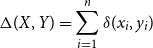 \begin{equation*}\Delta(X,Y) = \sum_{i=1}^{n}\delta(x_i,y_i)\end{equation*}
where
 \begin{equation*}\delta(x_i,y_i)=\begin{cases}\frac{x_i - y_i}{\max_i - \min_i} & \text{if numeric, otherwise}\\[4pt]0 & \text{if $x_i = y_i$}\\[4pt]1 & \text{if $x_i \neq y_i$}\end{cases}\end{equation*}
All features are nominal, both for WIN and PAR, meaning that according to the above equation, a comparison of any two features yields a value of 0 in case of an exact match (i.e. overlap), and 1 otherwise (i.e. no overlap). We illustrate this for sentences (3) and (5). Starting with the WIN approach, we can see from Table 1 that these sentences (rows one and four) have two feature values in common, viz. is in the L1 position and een in the R1 position. The other eight features all have different values, resulting in a distance of
 $2 \times 0 + 8 \times 1 = 8$
. For the PAR approach (Table 3), both instances share only one feature, viz. the Verb feature is. In this case, as three out of four features are mismatches, the distance is equal to
$2 \times 0 + 8 \times 1 = 8$
. For the PAR approach (Table 3), both instances share only one feature, viz. the Verb feature is. In this case, as three out of four features are mismatches, the distance is equal to
 $1 \times 0 + 3 \times 1 = 3$
.
$1 \times 0 + 3 \times 1 = 3$
.
The overlap metric as illustrated here is TiMBL’s most basic implementation of similarity/distance between instances, but other, more fine-grained metrics can be used as well (e.g. character-based measures like Levenshtein distance). In addition, the example above assumes that each feature is equally important, but this needs not be the case, and various feature weighting methods are available. The task of hyperparameter selection is discussed in Subsection 5.1 below.
In view of the hypothesis that the ND distribution of er is determined by stronger lexical collocation, whereas BD speakers need additional higher-level cues (cf. Section 2), we predict for RQ2 that the WIN approach works better for ND, while it is less suited for BD. Conversely, BD can be expected to gain more from syntactically informed lexical information compared to ND, so one could expect the PAR approach to yield comparatively better results for BD.
5. Analyses
5.1 Experimental setup
As indicated in Section 3, TiMBL operates with a number of hyperparameters, including the number of nearest neighbors taken into account for extrapolation (k), the similarity metric (m), the feature weighting metric (w), and the distance weighting metric (d). In addition to using TiMBL’s default parametric settings (
 $k = 1$
,
$k = 1$
,
 $m =$
overlap,
$m =$
overlap,
 $w =$
gain ratio,
$w =$
gain ratio,
 $d =$
no weighting), one can opt to use one or more non-default values in the function of a higher classification accuracy (cf. Hoste et al. Reference Hoste, Hendrickx, Daelemans and van den Bosch2002).
$d =$
no weighting), one can opt to use one or more non-default values in the function of a higher classification accuracy (cf. Hoste et al. Reference Hoste, Hendrickx, Daelemans and van den Bosch2002).
We wanted to take the influence of varying hyperparameter settings into account by iteratively using different combinations of hyperparameters from the possibilities in Table 5. Note that these do not exhaust all possible values; for m, w, and d, we selected the best-performing settings from earlier experiments in which we used van den Bosch’s (Reference van den Bosch2004) wrapped progressive sampling algorithm Paramsearch for automatic hyperparameter optimization.Footnote f For k, we selected values between 1 and 30, with increments of 5.
Table 5. Selected values for the TiMBL hyperparameters

The TiMBL experiments were carried out along two principal dimensions. The first dimension pertains to the respective feature representations for each national variety—window-based (WIN) versus parse-based (cf. Subsection 4.2). The second dimension involves the varieties, both in the training data and in the test data. Intra-varietal experiments (viz. training and testing within the same language variety) were contrasted with cross-varietal experiments (viz. training on the one variety and testing on the other), in both the WIN and the PAR approach. Following RQ3, we carried out this cross-varietal training because an additional way of gauging the syntactic individuality of BD and ND is measuring to what extent we can learn er-choices in the one variety on the basis of training material from the other.
Finally, we let sample size vary between 50 and 500 instances with and without er, with increments of 50. We did this because there is no way to know a priori how many instances the classifier needs to pick up on certain patterns in the data which are cues to er’s appearance. Each individual constellation of hyperparameters, feature representation, training and test variety, and sample size was repeated 10 times, each time randomly picking new training and test items from the balanced datasets, yielding 201,600 TiMBL runs in total.
5.2 Results and discussion
The results of the 201,600 experiments are visualized in Figure 3, by means of boxplots (with each box representing 2520 experiments). The four panels depict the two main experimental dimensions introduced in the previous section: on the horizontal axis, the WIN approach is contrasted with the PAR approach, while the vertical axis captures the distinction between intra- and cross-varietal training and testing. In each panel, the y-axis represents the accuracy (with the gray dashed line indicating the baseline of 0.5), while increasing sample sizes are plotted along the x-axis. The BD predictions are plotted in dark gray and the ND ones in light gray.

Figure 3. Boxplots capturing the accuracy for increasing sample sizes, both for WIN versus PAR feature representations and intra- versus cross-varietal training and testing.
First, across all four conditions (WIN and PAR, intra-varietal and cross-varietal) and varying sample sizes, the MBL classifier is able to predict er-choice fairly well, both for BD (
 $M=0.717$
,
$M=0.717$
,
 $SD=0.105$
) and ND (
$SD=0.105$
) and ND (
 $M=0.731$
,
$M=0.731$
,
 $SD=0.107$
). These findings demonstrate that a learning algorithm which relies on no more than lexical input can rival sophisticated regression analysis with researcher-defined abstract predictors. As such, RQ1, repeated here, can be answered positively: with a fairly straightforward implementation of bare lexical context, we are able to predict er’s distribution correctly in over 70% of the cases on average.
$SD=0.107$
). These findings demonstrate that a learning algorithm which relies on no more than lexical input can rival sophisticated regression analysis with researcher-defined abstract predictors. As such, RQ1, repeated here, can be answered positively: with a fairly straightforward implementation of bare lexical context, we are able to predict er’s distribution correctly in over 70% of the cases on average.
-
RQ1 Can a learning algorithm such as MBL learn the distribution of er in BD and ND on the basis of raw lexical input—and lexical input only—or does the classifier need linguistically enriched information?
Crucially, however, the accuracies are consistently higher for ND than for BD—at least in the intra-varietal experiments (cf. the top two panels in Figure 3). In the cross-varietal experiments, the difference is much smaller (cf. the bottom two panels, ibidem). In addition, the interquartile range in accuracy scores in the WIN approach is much smaller than in the PAR approach (cf. the left-hand panels versus the right-hand panels, ibidem), suggesting that a crude bag-of-word feature representation may in fact be slightly more predictive than a syntactically more informed representation such as PAR—at least in our implementation of it. This is especially the case for smaller sample sizes; with increasing sizes, the difference decreases.
In order to verify if the patterns in Figure 3 hold under multivariate control, we fitted a linear regression model predicting TiMBL’s accuracies while taking all significant
 $2\times2$
interactions between the hyperparameters (cf. Table 5) into account, as well as a three-way interaction between train/test variety, sample size, and feature type; polynomials of degree 3 were used for the predictors k and sample size (F(78,
$2\times2$
interactions between the hyperparameters (cf. Table 5) into account, as well as a three-way interaction between train/test variety, sample size, and feature type; polynomials of degree 3 were used for the predictors k and sample size (F(78,
 $201,521)=6657$
,
$201,521)=6657$
,
 $p<0.001$
;
$p<0.001$
;
 $R^2_{adj}=0.72$
). The effect plots in Figure 4 visualize the predicted accuracies resulting from the regression model, both for the WIN and PAR feature representations. The intra- and cross-varietal experiments are diagrammed together in order to allow for easier comparison. We have used different line types for the training varieties and different grayscales for the test varieties. The lighter bands around the lines indicate the 95% confidence intervals of the fitted values.
$R^2_{adj}=0.72$
). The effect plots in Figure 4 visualize the predicted accuracies resulting from the regression model, both for the WIN and PAR feature representations. The intra- and cross-varietal experiments are diagrammed together in order to allow for easier comparison. We have used different line types for the training varieties and different grayscales for the test varieties. The lighter bands around the lines indicate the 95% confidence intervals of the fitted values.
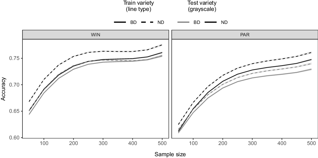
Figure 4. Effect plots for a linear regression model predicting TiMBL accuracies.
These results can be used to answer RQ2:
-
RQ2 Does the alleged lexical specialization of er in ND materialize in comparatively higher predictive success on the basis of raw lexical input than in BD? And, conversely, does the MBL analysis of er’s BD distribution require linguistic enrichment?
The fitted values plotted in Figure 4 reveal that, under identical conditions, the ND distribution of er (i.e. ND trained on ND, the black dashed lines) is comparatively easier picked up by the classifier than er’s BD distribution (i.e. BD trained on BD, the gray solid lines). Focusing on the left-hand panel (the WIN approach), it appears that ND does not need a lot of lexical training material—100 cases with and without er suffice—to attain accuracies of over 0.7, and the models quickly reach a saturation point in accuracy of 0.76 around a sample size of 250 +ER and 250 –ER cases. This is also borne out by the trend that can be discerned in Figure 3. The PAR approach initially lags behind, but the slopes are slightly steeper, and with higher sample sizes the difference decreases. This means that our earlier observation that WIN outperforms PAR should be reformulated more strictly: it does so, but only for small sample sizes. The rapid increase in accuracy with waxing sample sizes may be taken as an indication that the classifier actually benefits comparatively more from syntactically informed lexical information—given enough instances. It could be that PAR will, at some point, with still larger sample sizes, overtake WIN, but more data are needed to verify if this is actually the case.
However, contrary to our expectations, BD does not benefit significantly more from syntactically informed lexical information than ND: both in the WIN and PAR conditions, the ND models consistently outperform the BD models, although the latter only “lag behind” by about 2–3%.
Finally, we turn to RQ3:
-
RQ3 Does the lexical specialization which is hypothesized to streamline er-production in ND entail that the much “messier” BD data are less suited to learn er’s ND distribution? And, conversely, can a Belgian classifier learn er-preferences from the more “lexically entrenched” ND material?
Two important results can be pointed out here. The first one is that the ND data appear to be a slightly better training model for the BD distribution of er than the BD data, especially within the PAR condition, where the difference is much more outspoken (compare the gray dashed and solid lines). Second, when trained on BD data, the ND classifier performs somewhat worse compared to the cases where it is trained on ND data.
6. Error analysis
The foregoing experiments have demonstrated, on the basis of a large number of experiments, that MBL is quite able to discriminate between adjunct-initial sentences with and without er on the basis of lexical input which is not assigned to higher-level categories. To evaluate this success in a more qualitative way, we singled out two specific intra-varietal experiments (one BD and one ND) and zoomed in on the instances for which the presence or absence of er was incorrectly predicted by the classifier. On account of space limitations, we limit error analysis of the BD experiment to instances in which the classifier erroneously predicted +ER, while error analysis of the ND experiment is limited to cases where -ER was mistakenly predicted.
We first focus on a TiMBL-run with a BD 100-item test sample (50 +ER, 50 –ER) with window-based feature input and intra-varietal training, and parameter settings
 $m = J$
,
$m = J$
,
 $w = nw$
,
$w = nw$
,
 $d = ED1$
, and
$d = ED1$
, and
 $k = 25$
; resulting in an accuracy of 74%. There are 10 instances attested without er for which the classifier erroneously predicted er. In quite a few of these, like (8) and (9), the classifier’s confidence of inserting er hovers only slightly above 50%. Taking a closer look at the nearest neighbors which are responsible for the erroneous classifications, it becomes clear that a significant proportion of them have an adjunct constituent introduced by the preposition in “in” + the definite determiner de “the,” just like the target sentences, and a main verb which is often one of zijn “to be,” bestaan “exist,” and komen “come” (in its grammaticalized sense of “future existence”), which all frequently co-occur with er, as in (10) and (11) (the parts inside square brackets fall outside the window, so they were unavailable to the classifier).
$k = 25$
; resulting in an accuracy of 74%. There are 10 instances attested without er for which the classifier erroneously predicted er. In quite a few of these, like (8) and (9), the classifier’s confidence of inserting er hovers only slightly above 50%. Taking a closer look at the nearest neighbors which are responsible for the erroneous classifications, it becomes clear that a significant proportion of them have an adjunct constituent introduced by the preposition in “in” + the definite determiner de “the,” just like the target sentences, and a main verb which is often one of zijn “to be,” bestaan “exist,” and komen “come” (in its grammaticalized sense of “future existence”), which all frequently co-occur with er, as in (10) and (11) (the parts inside square brackets fall outside the window, so they were unavailable to the classifier).
-
(8) In de plaats komt_____ een nieuwbouw met vijf sociale [koopwoningen.]
in the place comes_____ a new_building with five social owner-occupied_homes
“Instead there will be a new building with five social owner-occupied homes.”
-
(9) In de leeftijdscategorie 15–49 jaar zapte____nagenoeg tien procent naar RTL.
in the age_category 15–49 years zapped____nearly ten percent to RTL
“In the age category of 15–49 almost ten percent watched RTL.”
-
(10) In de voorbije maanden waren er verschillende dergelijke verkoopdagen.
in the past months were there several such sales_days
“During the past months there were several sales days like that.”
-
(11) In de tweede fase komt er een aanpalende nieuwbouw.
in the second phase comes there an adjoining new_building
“In the second phase an adjoining new building will be built.”
Turning to the wrongly classified instances for which the classifier was much more certain, as in (12) and (13), a similar picture emerges. (For these, the classifier reports confidence scores of 83.1% and 77.7%, respectively.) In the case of (12), the vast majority of the nearest neigbors contains a form of the canonical er-booster zijn “to be,” which seems to be the most important trigger for TiMBL to insert er here. For (13), the nearest neighbors with er either also feature a form of zijn, as in for example (14), or another verb that expresses “existence” or “appearance” (cf. Grondelaers et al. Reference Grondelaers, Speelman, Geeraerts, Morin and Sébillot2002b, Reference Grondelaers, Speelman, Geeraerts, Kristiansen and Dirven2008, with reference to Levin Reference Levin1993) like blijven “stay, remain” and komen “come (into being), become,” in virtually all cases followed by the indefinite article een, as in for example (15).
-
(12) In de afgewezen plannen was_____plaats voor 36 eengezinswoningen.
in the dismissed plans was_____space for 36 single-family_dwellings
“In the dismissed plans there was space for 36 single-family dwellings.”
-
(13) Vanuit de Heidebloemstraat komt____een nieuwe straat om de [huizen in het
from the Heidebloemstraat comes_____a new street for the houses in the
Achterpad beter te ontsluiten.]
Achterpad better to open_up
“From the Heidebloemstraat there will be a new street for better opening up the houses in the Achterpad.”
-
(14) Aan de overzijde was er een attente Delva om De Wispelaere van een treffer te
on the other_side was there an attentive D. for D. W. off a goal to
houden.
hold
“On the other side there was an attentive D. to keep D. W. from scoring.”
-
(15) In sommige bedrijven bestaat er een systeem van buizen.
in some companies exists there a system of pipes
“In some companies exists a system of pipes.”
Let us move on to the 14 instances with incorrectly predicted -ER in the TiMBL-run on a ND 100-items test set with window-based input and intra-varietal training, parameter settings
 $m = J$
,
$m = J$
,
 $w = ig$
,
$w = ig$
,
 $d = IL$
, and
$d = IL$
, and
 $k = 20$
, and similar accuracy score of 73%. Classifications with a lower (
$k = 20$
, and similar accuracy score of 73%. Classifications with a lower (
 $< 60$
%) confidence score, like in (16), it becomes evident that two “classes” of neighbors are responsible for the misclassification. On the one hand, the nearest neighbors are almost all instances of frequent collocations like (geen) sprake zijn van and (geen) plaats zijn voor, of which four occur without er, and one with; examples (17) and (18). One the other hand, a heterogeneous group of verbs other than zijn occur without er, and occasionally also forms of zijn itself; for example (19).
$< 60$
%) confidence score, like in (16), it becomes evident that two “classes” of neighbors are responsible for the misclassification. On the one hand, the nearest neighbors are almost all instances of frequent collocations like (geen) sprake zijn van and (geen) plaats zijn voor, of which four occur without er, and one with; examples (17) and (18). One the other hand, a heterogeneous group of verbs other than zijn occur without er, and occasionally also forms of zijn itself; for example (19).
-
(16) Tijdens de Boekenmarkt zijn____optredens van straatartiesten en musici.
during the Book_Market are____performances of street_artists and musicians
“During the Book Market there are performances of street artists and musicians.”
-
(17) In de achttiende eeuw was geen sprake van contant geldverkeer [tussen
in the eighteenth century was no speech of cash monetary_transactions between
boekhandelaars onderling.]
booksellers mutually
“In the eighteenth century monetary transactions between booksellers were non-existent.”
-
(18) In een jongensdroom is geen plaats voor een cascade [van ongeluk.]
in a boy’s_dream is no room for a cascade of misfortune
“In a boy’s dream there is no room for a cascade of misfortune.”
-
(19) Onder de mogelijke tegenstanders was een aantal aanmerkelijk sterkere ploegen.
under the possible opponents was a number considerably stronger teams
“Among the possible opponents were a number of considerably stronger teams.”
As to the errors for which the classifier’s confidence score was high (
 ${>}80$
%), it becomes clear that a considerable group of them manifests a form of the verb ontstaan “arise, emerge, come into existence,” as in (20) and (21). Glancing at these sentences’ nearest neighbors, we may identify the verb as one of the crucial determinants of predicting -ER, which is mostly one of the posture verbs staan “stand,” hangen “hang,” liggen “lie,” and zitten “sit,’, as well as ontstaan itself and, once again, er-booster zijn; see (22)–(24). The choice of the posture verb strongly co-varies with the sentence-initial adjunct as well as the following subject: for example in (22) (urine)lucht “(urine) odor” is construed as “hanging” in the staircase (a vertical container), while the computer in the science lab in (23) is construed as “standing” on a horizontal surface (cf. Lemmens Reference Lemmens2002). In other words, the combination adjunct–verb in these cases may be strong enough a cue for the following subject that er is not needed.
${>}80$
%), it becomes clear that a considerable group of them manifests a form of the verb ontstaan “arise, emerge, come into existence,” as in (20) and (21). Glancing at these sentences’ nearest neighbors, we may identify the verb as one of the crucial determinants of predicting -ER, which is mostly one of the posture verbs staan “stand,” hangen “hang,” liggen “lie,” and zitten “sit,’, as well as ontstaan itself and, once again, er-booster zijn; see (22)–(24). The choice of the posture verb strongly co-varies with the sentence-initial adjunct as well as the following subject: for example in (22) (urine)lucht “(urine) odor” is construed as “hanging” in the staircase (a vertical container), while the computer in the science lab in (23) is construed as “standing” on a horizontal surface (cf. Lemmens Reference Lemmens2002). In other words, the combination adjunct–verb in these cases may be strong enough a cue for the following subject that er is not needed.
-
(20) [In de 10.000 meter] tussen Waarbeke en Meerbeke ontstond____een onvergetelijk
in the 10,000 meters between W. and M. emerged an unforgettable
achtervolging.
pursuit
“In the 10,000 meters between W. and M. an unforgettable pursuit started.”
-
(21) Tijdens de wedstrijd ontstond___onenigheid over een beslissing.
during the game arose disagreement about a decision
“During the game there was disagreement about a decision.”
-
(22) In het trappenhuis hangt een sterke urinelucht.
in the stairwell hangs a strong urine_odor
“In the stairwell there is a strong urine odor.”
-
(23) In een hoek van het laboratorium staat een computer.
in a corner of the laboratory stands a computer
“In a corner of the laboratory stands a computer.”
-
(24) Rondom het aardgas ontstond een industriële enclave, met alle onevenwichtigheden
around the natural_gas arose an industrial enclave with all imbalances
van dien.
of that
“Around the natural gas an industrial enclave arose with all its imbalances.”
While the accuracies reported in Section 5 demonstrate that MBL is quite successful in predicting presence and absence of er from bare lexemes which are not assigned to the higher-level categories, the error analyses in this section have shown that it may fail in cases where informative lexemes such as the verb are polysemous, or in cases where certain lexemes tend to form frequent collocations (e.g. (geen) sprake zijn van, (geen) plaats zijn voor) or otherwise predictive “chunks” (e.g. specific adjunct–verb, verb–subject, or even adjunct–verb–subject combinations). In the experiments reported here, each feature was considered independently. One evident way to account for subtle interrelations between features (i.e. lexemes) is by adding metrics that quantify their degree of attraction (see Evert Reference Evert, Lüdeling and Kytö2009; Gries Reference Gries2013), or proximity in semantic vector space (Lin Reference Lin1998; Turney and Pantel Reference Turney and Pantel2010).
7. Conclusion
In this article, we have reported a series of MBL experiments (Daelemans and van den Bosch Reference Daelemans and van den Bosch2005) to gauge the complex syntactic relationship between the two European national varieties of Dutch, viz. BD and ND. Previous data-driven research on this topic almost exclusively relied on regression modeling with researcher-defined higher-level features. Building on earlier research on existential constructions with er “there” (e.g. Grondelaers et al. Reference Grondelaers, Speelman, Geeraerts, Kristiansen and Dirven2008), we have shown that, instead of aggregating over individual instances by means of higher-level syntactic, semantic and pragmatic predictors, it is possible to discriminate between er-less sentences and sentences with er on the basis of immediate lexical input using MBL.
Using data from two Dutch newspaper corpora, we constructed two different types of datasets to test this: one in which each instance was stored as is, and one in which for each instance a number of syntactically and functionally informed lexical features derived from dependency parses were extracted which are known to be strong determinants of er’s distribution.
Crucially, we found that ND er-choices are easier to learn from raw lexical input than BD choices. The fact that MBL rivals regression modeling of er-choices in ND suggests that ND does not need researcher-defined higher-order features to attain optimal accuracy (cf. Theijssen et al. Reference Theijssen, ten Bosch, Boves, Cranen and van Halteren2013). The only possible explanation for this finding is the fact that syntactic choice seems to have become more collocation-based for ND than for BD, viz. driven by collocations between er and specific lexemes. This finding converges with Pijpops’s (Reference Pijpops2019) analysis of the competition between nominal and prepositional objects in Dutch, as with the verb verlangen “desire, long for” in (25)–(26), which turns out to be more lexically conventionalized in ND than in BD (examples from Pijpops Reference Pijpops2019, p. 188).
-
(25) Mannen verlangen eigenlijk maar drie dingen van een auto: […].
men desire actually just three things from a car: […]
“Men really only desire three things from a car: […].”
-
(26) Zo’n man verlangt naar kleine dingen: […].
such_a man desires to small things: […]
“Such a man desires small things: […].”
In RQ2, it was predicted that MBL models of BD benefit more from the introduction of “linguistically informed” features than MBL models of ND do. This prediction was not confirmed by the experiments. When interpreting these results, we should bear in mind that only one “linguistically informed” type of feature was tested. The features we used, viz. the lexical heads of the syntactic constituents that were deemed most important in the alternation pattern, arguably are still rather close to the pure lexical information. It may very well be the case that the BD classifier missed some important higher-level information which is not present in the raw lexemes, related to the subject’s contextual predictability and its concreteness, for instance (Grondelaers et al. Reference Grondelaers, Speelman, Drieghe, Brysbaert and Geeraerts2009). On the other hand, lexical input alone does not suffice to grasp er’s BD distribution equally well, not even when these lexical features are selected on the basis of higher-level syntactic information, meaning that in BD there are probably other interfering factors at play. Still, the results presented in this paper suggest that in BD, too, some lexical fixation effects have emerged. If that is indeed the case, it is clear why the ongoing lexical fixation of er-preferences in BD is easier to train from the even more fixated ND, but not vice versa (RQ3).
A potential limitation of the study reported here are the relatively small sample sizes. We preferred manual control over automatically generated datasets, which inevitably contain a certain degree of noise. We currently do not have clear intuitions as to why the curves already seem to flatten with a limited amount of training data. However, this question can be the topic of follow-up research, in which (much) larger, potentially automatically generated datasets can be put to the test.
The second avenue for future research is the exploration of alternative classification methods. Given the sequential nature of the classification task, a language model-based approach might be a viable option (e.g. RobBERT, a Dutch neural-network-based language model; Delobelle, Winters, and Berendt Reference Delobelle, Winters and Berendt2020).Footnote g However, for this study, we have chosen a memory-based approach, which gives us the advantage of interpretability. That is, in addition to attaining a reasonable classification accuracy, we think it is at least equally important for our purposes to understand the machinery behind the classification: which (type of) features co-determine the choice for er, and under which conditions (i.e. which constellation of hyperparameters)?
If anything, the data reported here occasion suspicion with respect to claims that the national varieties of Dutch have an identical syntactic motor. Although we have reported analysis of only one variable, there are striking indications that the grammars of the (European) Dutch national varieties differ from one another in an evolutionary perspective which merits and urgently requires further investigation. In ongoing follow-up research, we are currently focusing on the bottom-up extraction of hitherto unknown national variation in the grammar of Dutch, which will subsequently be tested with logistic regression and MBL tools to determine the division of labor between higher-order and lexical constraints in the syntactic makeup of BD and ND. In view of this, one obvious follow-up extension of the research reported here is a more systematic comparison of regression analysis and MBL. Another avenue of further research is the inclusion of measures which pertain to the subject’s predictability. Even without these extra features, the present paper has shown that an unsupervised machine learning algorithm is quite capable of handling one of the most notoriously complex phenomena in the Dutch grammar.


 Open access