


Introduction
The large-scale monitoring of facies on glaciers and ice sheets has become feasible in recent years through the advent of polar-orbiting, microwave remote-sensing satellites. Satellite synthetic aperture radar (SAR) has, in particular, the spatial resolution and all-weather operating capabilities necessary to monitor these facies routinely and in detail. The applications of this activity include hydrological planning (particularly in areas where glacier-fed melt is a significant contributor to total runoff) and early detection of CO2-derived and polar-enhanced changes in climate. In this paper, the potential of SAR for monitoring ice facies is explored with reference to two regions: the Wrangell Mountains of south-central Alaska and the west of the Greenland ice sheet.
Glacier Facies
Glacier facies are distinct zones in the surface layer of an ice sheet or glacier. These facies are related to patterns of accumulation and ablation and are illustrated in Figure 1, reproduced from Reference BensonBenson (1996). Benson's work, first published in 1962, was pioneering in first drawing attention to the pattern of glacier facies on the Greenland ice sheet. His work used a large number of ground survey points to interpolate a map for the facies over the island. Although the accuracy of the boundaries may be relatively poor in some locations, his maps are based on ground surveys with interpolation, so along the ground-survey profiles the boundaries should be accurate (for the time of the surveys). Since then, Reference Fahnestock, Bindschadler, Kwok and JezekFahnestock and others (1993) and Reference Long and DrinkwaterLong and Drinkwater (1994) have used a SAR mosaic and enhanced scatterometer data, respectively, to generate updated versions of the map generated by Benson. We begin this paper with a review of these facies.

Fig. 1. Glacier facies on an ice sheet, from Reference BensonBenson (1996)
Dry-snow facies
This facies is found only on the highest parts of ice sheets and some high-latitude glaciers. There is no surface melting in these regions and so the surface, consists of snow which is gradually compacted under its own weight, or metamorphosed under the effect of wind or depth-hoar development. The area is extensive over Greenland, but not necessarily uniform. In fact, recent studies (e.g. Reference Fahnestock, Bindschadler, Kwok and JezekFahnestock and others, 1993) indicate that there are systematic variations in this facies from southwest to northeast across Greenland. These regional differences may be related to corresponding variations in patterns of accumulation and wind leading to different morphological conditions in the snow, but this has not been established. The lower boundary corresponds approximately to the mean -5°C isotherm during the melt season (Benson, 1996, p.61), but according to Benson the boundary may be in the form of a 16-32 km wide transition region.
In general, SAR senses the dry-snow facies as a very dark region, as the grain-size of fresh snow is small compared to the wavelength of the C-band SAR systems (about 5 cm). Snow grain diameters above the wet-snow line are generally <5mm in diameter, with an approximate mean of 0.5-2 mm (Benson, 1996, Fig. 18). In the dry-snow facies, melting will not be a factor in the backscatter coefficient (?°). Any variations in ?° may be expected to derive largely from differences in grain-size. It is possible to derive a simple expression which, crudely, predicts the backscatter as a function of the grain-size. The backscatter coefficient for dry-snow, ?°ds, can be defined as follows:

where T 1 and T 2 are the transmission coefficients in the downward and upward directions, N is the number density of scattering elements, {|f i|2} is the scattering amplitude of a single element in the backward direction (for monostatic scattering), ? is the extinction coefficient, ??i is the refracted incidence angle and h is distance (Reference Partington and HannaPartington and Hanna, 1994). Assuming an effective transmission coefficient in both directions of 1, a uniform size of scatterers and a half-space, the above equation can be simplified to:


where is the dielectric constant, r is the particle radius and ? is the wavelength (Ulaby and others, 1981, cq. 5.85). The extinction coefficient, ?, is defined as follows, under the assumption that the absorption coefficient is dominant (Ulaby and others, 1981, eq. 5.100):

By substituting Equations (3) and (4) into Equation (2), the following is derived:

which for ERS-1 (? = 0.056, ? i = 23°) and assuming a dielectric constant of 3.15 - 0.0025j, simplifies to
Equation (6) suggests that the backscatter coefficient would range from -20 dB for a grain mono-distribution with mean radius of 0.25mm to -2 dB for mean grain radius of 1 mm.
It must be stressed that this is a crude approximation which neglects multiple scattering, but it provides an indication of the sensitivity of the SAR to systematic variations in grain-size, which may be related to regional variations in accumulation rate and temperature. This equation will not help to interpret the effects of rime-frost, depth hoar or other complex physical phenomena.
Percolation facies
Here, the surface snow is occasionally subject to melt which results in the percolation and refreezing of meltwater in the form of pipes and lenses (see Reference Ahlmann and sonAhlmann, 1935; Reference SharpSharp, 1951; Reference Marsh and WooMarsh and Woo, 1984), There may be no clear surface manifestation of the boundary between this facies and the dry-snow facies. The percolation facies can, however, consist of significant bodies of ice. Reference Echelmeyer, Harrison, Clarke and BensonEchelmeyer and others (1992) found a 5 cm thick layer of ice at 30 cm depth in this facies, with grains typically 1-2 mm in diameter. C. S. Benson (personal communication) has recorded photographs of pipes corresponding to a percolation facies in Alaska, where dimensions are typically 10 cm long and a few cm diameter. Over Greenland, K. G Jezek (personal communication, 1996) found that sizes of inclusions vary appreciably. At Crawford Point (just inland from Jakobshavn in the percolation facies), massive ice pipes tens of centimetres long and up to 10 cm wide were found. Once out of the jakobshavn drainage area, but still at about the same elevation, Jezek found that the ice-pipe sizes decreased dramatically to about 10 cm long and 2 cm wide, which seemed characteristic all the way up to the Dye 2 site (66.5° N, 46.3° W). At Dye 2, smaller isolated lenses were found.
The presence of ice pipes and lenses can act to increase the backscatter in SAR data substantially over that commonly found in the dry-snow facies. Ice lenses and pipes can have dimensions comparable to the wavelength of the SAR and so can produce high returns. This is confirmed by Reference Fahnestock, Bindschadler, Kwok and JezekFahnestock and others (1993), who note from their SAR mosaic of Greenland that there is a sharp contrast between the backscatter from the centre of Greenland (low) and the percolation facies which surrounds it (high). Based on the observations of K. C. Jezek (personal communication, 1996) and Reference BensonBenson (1996), it may be expected that there would be a smooth gradation of backscatter from the dry-snow facies to the percolation facies, rather than a sharp boundary, and this is confirmed by Reference Fahnestock, Bindschadler, Kwok and JezekFahnestock and others (1993).
Wet-snow facies
The wet-snow facies is defined as extending further down the glacier from the point in the percolation facies at which the entire annual accumulation of snow is subject to melt and refreeze. In this facies, the snow mass reaches melting point as a result of latent heal released by extensive refreezing of meltwater. As a result, grain-sizes are larger and re-crystallisation is the norm rather than the exception. The transition to the wet-snow facies from the percolation facies takes place over a few kilometres, according to Reference BensonBenson (1996). In general, the wet-snow facies will be damp throughout the ablation season, although refreezing at the surface will occur. In the lower altitudes of the wet-snow facies there may be lakes and areas of slush where melting is particularly vigorous.
During the ablation season, the wet-snow facies will reduce markedly in backscatter intensity, and the main scattering mechanisms will alter. The penetration depth of dry snow at the configuration of the ERS-1 SAR (C-band) is of the order of 20 m (Ulaby and others, 1981, Fig. 11.25). Very small amounts of moisture drastically reduce the penetration depth, so that a volumetric moisture content of2% will reduce the penetration depth to approximately 1 % of its dry equivalent (Reference Ulaby, Moore and FungUlaby and others, 1981). The scattering mechanism will therefore change from predominantly volume scattering to surface scattering. Ulaby and others (1986, p. 1893) note that at G-band, the Fresnel reflectivity at normal incidence for snow with 10% liquid water is 0.06. Using this, the Kirchhoff Geometric Optics model predicts that, with an rms slope of 0.2-0.4 the backscatter coefficient ranges from -9.6 to 16.2 dB, which is similar to, or even considerably less than, the backscatter expected from the dry-snow facies (Ulaby and others, 1986, eq. 21.27). Thus, we would expect the darkest, areas in a SAR image of glaciers to correspond to damp areas. A layer of damp snow under refrozen or fresh, dry snow would show little difference in backscatter as a result of the high penetration depth of radar in dry snow.
There is little reason to suppose that the wet-snow facies will show fundamentally different scattering mechanisms to the percolation facies, except during early and late summer when the melt limit is moving up- and downslope, respectively. However, Reference Fahnestock, Bindschadler, Kwok and JezekJezek (1993) found that the backscatter from the wet-snow facies was much more strongly varying than from the percolation facies. The slush which can form at the base of the wet-snow facies can cause dark patches to appear in the SAR image data (Reference Bindschadler and VornbergerBindschadler and Vornberger, 1992). In addition, it may be expected that there will be a general gradation of mean backscatter with altitude as a result of the change in density and size of lenses and pipes. Nevertheless, the wet-snow line may not be expected to be detected as a discrete boundary as it can have no influence on the sensing properties of the SAR, the line being coincident with the subsurface position where the 0° isotherm reaches the base of the previous year's accumulation, and so hereafter in this paper the percolation and wet-snow facies are treated together.
Superimposed-ice zone
Below the wet-snow facies, but still within the general accumulation area of the ice sheet, there may lie a region of superimposed ice, which is high-density refrozen melt from the previous year's accumulation. In a heavy ablation year, this facies may not exist, as the ice may be completely melted, leaving the snowline equivalent to the equilibrium line (the boundary between net accumulation and net ablation). In a lighter ablation year the equilibrium line will lie between the superimposed-ice and ice facies, giving it a different surface manifestation. G. Marshall (personal communication, 1995) suggests that the superimposed-ice facies is potentially distinguishable in SAR data as a result of its greater degree of smoothness relative to the ice facies.
Ice facies
The lowest part of an ice sheet or glacier consists of the ablation region, or ice facies. Here, the total year's accumulation, and more, is lost to melting. During winter, the ice facies will be covered by dry snow. During early summer, the snow will be melting so that by the end of the ablation season the entire accumulation of snow will have been melted, as will some of the ice from previous years' accumulation. The backscatter from SAR is likely to decrease slowly-through winter as the relatively rough ice snow interface becomes buried by attenuating dry snow (which itself generates very little backscatter). When the snow melts, the backscatter will decrease further, as was indicated above for the wet-snow facies. Once the snow has melted, leaving bare ice, the backscatter is likely to reach its yearly peak as a result of exposure of a rough, dense ice surface.
Study Objectives
The aim of this study is to carry out a detailed analysis of the extent to which glacier facies are visible in SAR data and to achieve this through the use of multi-temporal SAR image data.
The approach taken has been to combine SAR images from three parts of the season: winter, early summer and late summer (end of the ablation season). The two key images are the first and last of these. The winter image defines maximum freeze conditions, and the late-summer image defines maximum melt conditions. The timing of the first of these is non-critical, as during winter the backscatter signatures from the different glacier facies change little. The timing of the late-summer image is important, as conditions change rapidly at this time. One approach in glacier monitoring is to select a single date and define this as the end of the ablation season, ignoring annual variations in the timing of the actual end of the ablation season. The date selected here is around the end of August/beginning of September.
By co-registering the three SAR images, then mapping the three images to red, green and blue channels of a three-band image and displaying the result, it is possible to see multi-temporal signatures displayed as distinctive colours. Some of the multi-temporal signatures are quite subtle and would not be at all obvious from comparison of the three individual images by eye. In this paper, it is demonstrated that the patterns of distinctive multi-temporal signatures found in a three-band multi-temporal SAR image of a glaciated region reflect the distribution of glacier facies, and so the three-band SAR image effectively provides a mapping of glacier facies.
The power of multi-temporal observations of glaciers is demonstrated with reference to two test areas, West Greenland (71°30? 76°30?N) and the Wrangell-St Elias Mountains, south-central Alaska, with satellite data collected during 1992-93 in each area. The two test sites are quite distinctive in terms of topographic settings and climate regimes, which is intentional and designed to demonstrate the wide utility of this technique.
The following specific questions are addressed in this study:
-
What facies are visible in multi-temporal SAR imagery collected from winter, early summer and late summer?
-
What techniques can be used to extract information on these facies?
-
What do these techniques tell us about conditions during 1992-93 in the two test areas of West Greenland and the Wrangell St Elias Mountains?
Study Areas and Data
The two test areas are shown in Figures 2 and 3.


Fig. 3. Map of the Alaska (Wrangell) test area, showing coverage of Figure 7
Greenland
The Greenland test area, for june 1992 January 1993, corresponds to a 100 km wide and 600 km long SAR swath (generated using six neighbouring image frames) extending from the west coast at 71°30?N, 53° W, well into the dry-snow facies at approximately 71°30? N, 43° W. The coverage includes several outlet glaciers which extend to sea level and calve icebergs. Major glaciers include (from north to south) Umiámáko Isbræ, Rink Isbræ and Kangerdluarssp sermia. These "major" glaciers have widths at their seaward margin of 5-10 km. Many smaller glaciers are also present.
There are supporting data for the study. Meteorological data provided by H. Rott of the University of Innsbruck were recorded at Godthåb/Disko (sea level). These give the air temperature and dew point at 1200 h for dates relevant to the acquisition of image products. Table 1 summarises the relevant supporting data.
Table 1. SAR image data and associated meteorological observations from Godthåb/Disko (sea level)

As well as measurements of conditions at the time of the acquisition of data, there are the results of field surveys which provide estimates of the altitudes of glacier facies between 69° and 70° N (Table 2).
Table 2. Estimated altitudes (m) of glacier facies, from field measurements (for approximately 69° N, west coast of Greenland)

Alaska
The Wrangell-St Elias Mountains in south-central Alaska contain a high density of glaciers and, as a result of the fairly high latitude and altitudes (62° N, peaks greater than 4000 m a.s.l.), some of the glaciers have a complete range of glacier facies from dry-snow facies downwards. Lingle and others (in press) have undertaken a study of Nabesna Glacier in which they show that the snowline and terminus positions are clearly evident in winter ERS-1 SAR data. A set of three ERS-I images is available from the study for this area, recorded at very similar times of year to those from Greenland, to make the multi-temporal images broadly comparable.
Study Techniques
Overview
Figure 4 illustrates the processing used to generate the multi-temporal, three-band SAR data. The three SAR images (from winter, early summer and late summer) are calibrated, co-registered (i.e. registered to each other), terrain-corrected (in the case of the Alaska data only) and combined to Form a multi-temporal SAR image, which can be displayed as a colour image. This colour image is used to provide a visual map of distinctive multi-temporal signatures which are related to glacier facies. Furthermore, quantitative analysis is carried out using the Alaska data, where a co-registered digital elevation model (DEM) is available to map profiles of multi-temporal signatures (backscatter coefficients) as a function of both altitude (along Nabesna Glacier) and slope orientation (near the summit of Mount Wrangell).

Fig. 4. Flow diagram showing the technique used for generating multi-temporal, three-band SAR image data. The Alaska multi-temporal SAR products were generated using tools which are available from the Alaska SAR Facility Website, http://www.aifalaska.edu/
Table 3. SAR data for the Wrangell-St Elias test site

Pre-processing
The SAR data were all recorded by the European Space Agency (ESA) ERS-1 satellite during 1992-93. Three images were selected, providing single observations from winter, early summer and late summer. The SAR data were selected to be almost exact repeat data. That is, the data are separated by a multiple of the repeat-cycle period of the satellite so that the observation geometry is almost identical. This is important, as any significant difference in observation geometry associated with the three SAR images would create backscatter differences which were related to observation geometry rather than seasonal change.
The SAR data are first calibrated using the full calibration procedure recommended by ESA (summarised in Reference Laur, Bally, Meadows, Sanchez, Schaettler and LopintoLaur and others, 1996), except for power-loss correction which, as a result of the averaging required, can create artificial discrete changes in backscatter across frame boundaries (which is a problem here as image mosaics are being used). The lack of a power-loss correction does not affect most of the analysis, as we are concerned with changes in backscatter coefficient and backscatter ratios between dates rather than absolute levels of backscatter.
The SAR data are then geo-referenced into Universal Transverse Mercator (UTM) projection and co-registered to common boundaries and pixel spacing, so that any arbitrary pixel in one image corresponds in location on the ground to the same pixel position in the other two images of the same area, and north corresponds to the vertical axis. The Alaska SAR data were resampled to 90 m pixel spacing, which corresponds to the pixel sparing of the DEM used to terrain-correct the data.
In order to provide coverage of all glacier facies, six SAR image frames from Greenland were mosaicked together to create a long 100 km by 600 km strip of data which stretches from the coast well into the interior of the ice sheet. As a result of the large coverage, the Greenland SAR data were resampled to 1 km pixel spacing. Mosaicking was not carried out for the Alaska data, as all glacier facies were covered in a single SAR image.
Following mosaicking, the calibrated, geo-referenced and co-registered SAR data may be terrain-corrected using a DEM. This corrects for distortions in the topography caused by the imaging geometry of the SAR, whereby mountain peaks "lean" towards the near-satellite side of the image. In practice, this procedure was carried out for the Alaska data only, as a suitable DEM was not available for the Greenland data. For the Alaska data, digital elevation data are available from the U.S. Geological Survey (USGS), at a pixel spacing of 90 m, and these data were used to terrain-correct the SAR images for the Mount Wrangell region. The calibrated, geo-referenced, co-registered and terrain-corrected images from the Mount Wrangell region are shown in Figure 5. North is towards the top of each image, and the area covered by each image is approximately 50 km by 50 km (some of the original SAR image coverage has been cropped).

Fig. 5. Terrain-corrected, map-projection ERS-1 image segments of Mount Wrangell and the area to the east, with north towards the top of the figure. For the location of Mount Wrangell and Nabesna Glacier, see Figure 7.
Formation of multi-temporal, colour SAR images
Figure 4 shows that once the images have been calibrated, geo-referenced, co-registered and (optionally) terrain-corrected, they are merged by creating a single three-band image in which (arbitrarily) the blue channel to the winter image, the red channel to the early-summer image and the green channel to the late-summer image.
The actual colour displayed in the multi-temporal image will depend on the form of the multi-temporal signature, and Figure 6 shows how the displayed colour relates to the form of the multi-temporal signature in the three-band SAR image. If the backscatter in winter is much larger than the backscatter in early or late summer, then the multi-temporal image will appear blue. A lack of colour (black, grey, white) indicates very little difference in the backscatter on all three dates. A non-primary colour (e.g. purple) indicates that backscatter is high on two dates (in this case winter and early summer) and low on the third date (in this case late summer).

Fig. 6. Diagram showing the relationship between backscatter coefficients on the three dates (30 December 1992, 23 June and 1 September 1993) and colour in the multi-temporal SAR images. The vertical bars indicate backscatter coefficient. This figure may be used to reference the meaning of colours in Figures 7-9
Results
The colour schemes for the Greenland and Wrangell data are equivalent (blue = winter, red = early summer, green = late summer), and the resulting multi-temporal, three-band SAR images are displayed for the Mount Wrangell region in Figure 7 and for West Greenland in Figure 8. In Figure 8, contours of backscatter differences, in dB, between 23 June 1992 and 16 January 1993 are given inland of the coastal region (the coast is the lower, left side of the diagram). It can be seen from both the contours and the lack of colour that nearly the whole area in Figure 8 shows no significant multi-temporal signature. This is expected, as most of the region consists of the dry-snow facies, which appear as dark grey, and the percolation facies, which appear as white. However, there is significant temporal variation in backscatter in the coastal region and this is shown expanded in Figure 9. Recall that the dates of the component images (winter, early summer and late summer) in Figures 7-9 are given in Tables 1 and 3 and that the SAR data are terrain-corrected in Figure 7 but not in Figures 8 and 9.

Fig. 7. Terrain-corrected, map-projection multi-temporal ERS-1 image segment of Mount Wrangell and the area to the east, with north towards the top of the figure. Blue indicates data from 30 December 1992, red indicates 23 June 1993 and green indicates 1 September 1993. The background yellow-green signature in non-glaciated areas indicates a marginal increase in backscatter during the summer months which is thought to reflect growth of vegetation. The blue profile (A) shows the location of Figure 10, and the red profile (B) shows the location of Figure 11. Numbers refer to altitude above sea level, in metres.

Fig. 8. Multi-temporal image mosaic of Greenland. The image is in map projection, with north at the top of the figure. Blue indicates data from 16 January 1993, red indicates 20 June 1992 and green indicates 29 August 1992. Contours indicate backscatter coefficient differences (dB) between the 20 June 1992 and 16 January 1993 images, except in the coastal region (bottom) where the difference is >0.2dB. Nearly the whole area covered by this figure corresponds to the percolation facies (bright) and dry-snow facies (dark) and so shows no significant multi-temporal signature.

Fig. 9. The coastal (lower) portion of the multi-temporal image swath from Figure 8 (expanded to show detail). The image is in map projection, with north as the top of the figure. Blue indicates data from 16 January 1993, red indicates 20 June 1992 and green indicates 29 August 1992. The approximate position of the coastline is indicated by a white line.
As digital elevation data are available for Mount Wrangell, it is possible to generate profiles of multi-temporal backscatter signature both as a function of altitude along the Wrangell Icefield-Nabesna Glacier from source to terminus and as a function of orientation close to the summit of Mount Wrangell (4000 m a.s.l.). These profiles are located in Figure 7 and can assist in determining the boundaries of the various facies and in analyzing their characteristics. Figure 10 shows profiles of the backscatter coefficients for 30 December 1992, 23 June 1993 and 1 September 1993 as a function of altitude, for a line down Nabesna Glacier. These profiles extend from the dry-snow facies down to the ice facies. Figure 11 shows profiles of the backscatter coefficients for the same dates around the summit of Mount Wrangell at 4000 m a.s.l., in the dry-snow facies.

Fig. 10. Backscatter coefficients vs altitude along Nabesna Glacier and up to Mount Wrangell, for the three different dates. See Figure 7 for location of profile.

Fig. 11. Backscatter coefficients as a function of orientation of slope at 4000 m.a.s.l. on Mount Wrangell and for the three different times of the year. See Figure 7 for location of profile.
In the following sections, the manifestations in the multi-temporal SAR data of each of the glacier facies are described and possible explanations provided.
Dry-snow facies
Over a very wide region of the Greenland test area (Fig. 8), the dry-snow facies can be located from a combination of low backscatter and the complete absence of any multi-temporal signature (dark grey in Figure 8). The radiometric stability (over the 7 months represented in this time series) is < ±0.2 dB over most of the mapped dry-snow area of 100 km x 300 km, which is an indication from a natural, uniform distributed target of the stability of the ERS-1 SAR which is well within the design criteria for the instrument. However, an area to the north of the test region shows higher variation, up to 0.6 dB, which may be related, in some way, to the lower accumulation rate in that region.
The area bounded by a calibrated backscatter coefficient of-8dB (after correction for power loss) corresponds very closely with the dry-snow facies as defined by Reference BensonBenson (1996) in this region and estimated using the supporting data provided in this study (i.e. dry-snow line at ~2400 m a.s.l.). However, the overall range of backscatter coefficient across the dry-snow region of Greenland appears to be a minimum of about -14 dB and a maximum of about -5 dB, judging from a comparison of the Greenland facies map of Reference Long and DrinkwaterLong and Drinkwater (1994) with a map of fully calibrated ERS-1 backscatter coefficient across Greenland generated by P. J. Meadows, in Reference SephtonSephton and others (1995) (which includes power-loss correction).
These variations in backscatter coefficient across the dry-snow facies may be related to regional differences in accumulation rates. Largest grain-sizes are found in areas of lowest annual accumulation, where they may reach 1-2.5 mm in radius, through a process of depth-hoar development (Reference PatersonPaterson, 1981). However, these values are unlikely to be attained with continuity, vertically through the snowpack. If these grain-sizes were continuous, the backscatter coefficient would reach a figure of the order of-2.5 dB (Equation (6)). More typical snow sizes are radii of the order of 0.5 mm for snow which has not been subject to depth-hoar development, suggesting a backscatter coefficient of-11 dB (Equation (6)).
In the Wrangell data (Fig. 7), the dry-snow facies is indicated by patchy, dark areas near the summit. There is much less stability between the observations at different times of the season here than in Greenland.
The following equation most closely maps the extent of the dry-snow facies determined by Reference BensonBenson (1996) at the latitude associated with (his test site:
This criterion gives a mean altitude for the dry-snow line around Mount Wrangell of approximately 3460 m on the north side and above 4000 m on the south side (from the September image data). This compares with an altitude of about 2400 m for the test area in Greenland (the precise altitude cannot be measured, as a result of a lack of elevation information).
Percolation and wet-snow facies
Reference Fahnestock, Bindschadler, Kwok and JezekFahnestock and others (1993) showed that the percolation facies tends to be bright in ERS-1 SAR image data. This is true of winter image data and the highest areas of the percolation facies. In summer, however, areas of melt can extend into the percolation/wet-snow facies, reducing the backscatter coefficient (to below -15 dB in the Wrangell region). Thus, in the multi-temporal images generated here, we would expect to sec high-backscatter winter image data combined with early- and late-summer image data which will show the passage of surface melt into the wet-snow/percolation facies. In general, we will expect to find three zones within the percolation/wet-snow facies displayed in Figures 7-9. At the highest altitudes (the "upper zone") we would expect to find a uniformly high backscatter coefficient for all three dates, as at the highest altitudes in the percolation Facies we would not expert to find melt on any of the three dates. This region would appear "white" in Figures 7-9. Further down (the "middle zone"), we would expect to find a region in which melt is present in the late-summer image but not in the early-summer or winter image. This region would appear "'purple" in Figures 7-9, as the backscatter will be uniformly high during winter and early summer and low in late summer. Finally, towards the lowest altitudes in the percolation/wet-snow facies (the "lower zone"), we would expect to find melt associated with both early- and late-summer images, so the backscatter would be high in the winter data and low in both summer images. This region would appear "blue" in Figures 7-9. This is summarised in Table 4.
The upper percolation/wet-snow facies (Table 4) is extensive in Greenland (Fig. 8, white areas), indicating widespread freezing conditions on all three dates. The backscatter coefficient is of the order of-4 dB. Interestingly, the stability for the three images is as high as that of the dry-snow facies (<0.2dB). Moving down towards sea level (Fig. 9), some very limited "purple" regions indicative of the middle zone in the percolation/wet-snow facies are encountered (suggesting melt in the August data, where backscatter reduces to -10 dB) and then the "blue" lower percolation/ wet-snow zone (indicative of melt in both the June and August data), The altitudinal limit of the combined lower mid middle percolation/wet-snow zones in Greenland corresponds closely with the estimated highest altitude of melt of 1080 m on 17 June and 23 July 1992 (Table 1).
This pattern of zones is reproduced on the north- and east-facing slopes of Mount Wrangell, in an entirely analogous progression to that found in the Greenland data. On the south-facing slopes, however, the "upper zone" of the percolation/wet-snow facies appears green instead of white. This indicates higher backscatter in September than in December or June. This "green" tint extends almost to the summit of Mount Wrangell on the south-facing slopes, and includes areas that have very low backscatter in winter and so would be classified from winter data as being in the dry-snow facies. In fact, although the upper area on the south-facing slopes has very low backscatter in winter and early summer, the backscatter increases markedly in late summer by more than 5 dB. The difference in multi-temporal signature as a function of orientation is shown very clearly in Figure 11, for an altitude of 4000 m a.s.l.
Table 4. Percolation/wet-snow facies, divided into "upper", "middle", and "lower" zones, which relate to either "freezing" or "melting" conditions associated with the winter, early-summer and late-summer SAR images. Summary of appearance by zone in Figures 7-9

This multi-temporal signature at high altitude on Mount Wrangell is extremely unlikely to be an instrument artefact, for the following reasons:
-
the imaging geometry is virtually identical, and in this situation the stability of ERS-1 is a few tenths of a decibel (Reference SephtonSephton and others, 1995). The observed temporal difference (September-June backscatter coefficient) is a maximum of 5dB for slopes facing south;
-
the signature is observed only on south-facing slopes and only in the percolation/wet-snow facies;
-
registration errors would create similar artefacts elsewhere through the image and, in any case, cannot be large enough to account for the areal coverage associated with this multi-temporal signature.
As there is no ground truth to validate an interpretation, possible explanations are offered here for future investigation. Three possible explanations are:
-
summer depth-hoar development;
-
rime-frost development;
high winter accumulation over percolation facies.
Depth hoar consists of large, faceted crystals which develop from sublimation in the presence of a strong vertical gradient in vapour pressure (Reference Giddings and LaChapelleGiddings and LaChapelle, 1962). The development of depth hoar is a function of both the maximum degree of heating during the day and the diurnal range of temperature (Reference ColbeckColbeck, 1989). This would be consistent with the fact that the multi-temporal signature is found on the south sides of Mount Wrangell and not on the north or east sides, where diurnal temperature ranges are much smaller in summer. By late summer, the surface is cooling rapidly at night but the subsurface pack is still relatively warm, setting up a strong temperature gradient conducive to the formation of depth hoar (Reference PatersonPaterson, 1981). During winter, the backscatter would reduce as this depth-hoar layer is covered by a considerable attenuating layer of snow which on Mount Wrangell exceeds 100 cm w.e. on average (Reference Benson, Bingham and WhartonBenson and others, 1975). Studies by Reference BensonBenson (1968) show that depth hoar develops on Mount Wrangell each summer, but there is no direct evidence that it is better developed, to the point of being detected by the SAR, on the south-facing sides.
Rime-ice layers are also predominantly summer features which appear on Mount Wrangell, but in this case not in response to high temperature gradients but rather in response to storms (Reference BensonBenson, 1968). These layers may also form preferentially on the south side of Mount Wrangell as storms move in largely from the south. It is not clear that these features would act to increase the backscatter markedly, although Reference BensonBenson (1968) does note the frequent occurrence of these summer features on Mount Wrangell in excavated snow pits.
High winter accumulation over the percolation facies is a third possible explanation for the seasonal signature at high altitude on the south-facing slopes of Mount Wrangell. The annual accumulation rate averages 100 cm w.e. in the caldera, which equates to approximately 320 cm of snow (Reference BensonBenson, 1968), but could be higher on the south-facing slopes than on the north- and east-facing slopes (given the direction ?f predominant storm tracks).
Without validating information, it is not possible to draw a firm conclusion on whether rime-frost, depth hoar or high winter accumulation rates are causes of this multi-temporal signature in the SAR data on the south-facing slopes of Mount Wrangell. All three are mentioned simply as possibilities.
Ice facies
The ice facies lies below the equilibrium line, which is present in the Wrangell data at about 2100 m (Lingle and others, in press). There is no evidence for or against the presence of superimposed ice in the Wrangell data. In Figure 7, the ablation region can be seen to lie below the "blue" lower zone of the percolation/wet-snow facies (e.g. along the Nabesna profile) and the ice facies appears as having a green tint in the multi-temporal data. This indicates higher backscatter in September than in June or December.
Bare ice exists at the end of the ablation season (September image), but earlier in the season there remains snow cover. As explained earlier, a deep, dry- or wet-snow cover has the effect of attenuating return from the relatively strong bare-ice scattering surface, hence the green colour indicative of relatively strong scattering in September, except in areas of moraine which can be identified by longitudinal streaks in the glacier showing no multi-temporal signature.
A definition for the snowline is proposed as follows:
where subscripts "s" and "d" indicate September and December, respectively. This places the snowline on Nabesna Glacier at about 2100 m a.s.l. This compares well with the figures provided by Reference BensonBenson and others (1996) from both SAR data and air photographic data from nearby MacKeith Glacier (where it is estimated as varying in altitude between 2090 and 2230 m a.s.l.). The mean backscatter coefficients for the altitude range 950–2000 m on Nabesna Glacier (the ice facies), are shown in Table 5.
The June backscatter is consistent with scattering from a damp-snow surface. The scatter from bare ice (in September) would be expected to be greater, as the surface is rougher but will still be damp in September. In December, the scatter will be from a dry, bare-ice surface and volume attenuated by a layer of dry snow. In this area, snow depths in December are typically of the order of 2 m (personal communication from C. S. Reference Benson, Lingle and AhlnaesLingle, 1996).
Table 5. Mean backscatter coefficients front the ice facies on Nabesna Glacier

An important implication of the Greenland data is that the percolation/wet-snow facies in these data extends to sea level in this region. There is no region in the Greenland data comparable to the ice facies visible in the Mount Wrangell data. This suggests a high-accumulation, or low-ablation year in 1992. Evidence in support of this result is provided by both Reference Thomas, Krabill, Frederick and JezekThomas and others (1995) and Reference Van Tatenhove, Roelfsema, Blommers and van VoordenVan Tatenhove and others (1995), who each note that 1992 was charaecerised by a very cold summer in West Greenland around Leverett Glacier and Jakobshavns Isbræ at 69° N. The average temperature at Kangerdlussuaq was 44°C from May to October, and 7.9° C from June to August, making it the fourth coldest summer between 1942 and 1992. Jakobshavns Isbræ thickened by several metres between September 1991 and April 1992 and, using aircraft-derived elevation profiles, Reference Thomas, Krabill, Frederick and JezekThomas and others (1995) found that, unusually, this was not compensated by summer melting during the following summer. Furthermore, Reference Abdalati and SteffenAbdalati and Steffen (1997) found, from passive microwave data, that there was a lack of melting during the summer of 1992 over Greenland as a whole, which they attribute to the eruption of Mount Pinatubo and the resultant increased aerosol concentrations in the atmosphere. In fact, the mean melt area (for the months of June, July and August over Greenland as a whole) in 1992 was about 0.7 x 10⁵ km2as opposed to mean melt areas during the summers of 1979-91 of about 0.9-2.25 105 km2 (Reference Abdalati and SteffenAbdalali and Steffen, 1997). Thus, there is strong evidence here, from a variety of sources, that ablation was unusally low in 1992, and the SAR data suggest that around 71° Non the west coast of Greenland die equilibrium line was at sea level at the end of summer that year.
Conclusions
This study has provided the following significant results.
A technique is described for combining SAR images from the middle and end of the ablation season with images from winter to locate glacier facies. The technique is simple but requires use of repeat SAR data, calibration, co-registration and, ideally, terrain correction and image mosaicking. Two parameters considered, in combination, to give the best positioning for the snowline and dry-snow line are winter backscatter coefficient and the difference between end-of-ablation and winter backscatter coefficients as shown in Figure 12. The resulting multi-temporal signatures are illustrated schematically in Figure 13, based on data from Nabesna Glacier but also showing corresponding points from the Greenland data. Use of absolute backscatter coefficients in combination with multi-temporal SAR signatures adds to the value of the data.
The dry-snow facies shows up clearly, although the boundary with the percolation facies is indistinct. A definition is suggested for the dry-snow line in SAR data.
Late-summer development of depth hoar, storm-produced rime-frost or high winter accumulation rates may account for slope-orientation-dependent facies differences on Mount Wrangell.
Damp snow shows up very clearly and its migration Up-glacier into the wet-snow/percolation facies can be followed. This migration allows a subdivision of the percolation/wet-snow facies into a lower, middle and upper zone.
For the data analyzed here, the altitudes of the snowlines are estimated, In West Greenland in 1992, at 71°30? N, the equilibrium line appears to be at sea level, indicating a low-ablation or high-accumulation year (Table 6). A low-ablation year is supported by evidence from a variety of sources. This interpretation is based on cross-comparison of multi-temporal signatures from the Wrangell and Greenland test sites, which shows the complete absence of an ice-facies signature in the Greenland data. This low-ablation year appears to be related to the eruption of Mount Pinatubo (Reference Abdalati and SteffenAbdalali and Steffen, 1997). A definition for the snowline in SAR data is suggested.

Fig. 12. Glacier facies illustrated by reference to September-minus-December backscatter coefficient (lefthand axis) and December backscatter coefficient (righthand axis) for Wrangell-Nabesna Glacier as a function of altitude. See Figure 7 for location of profile.
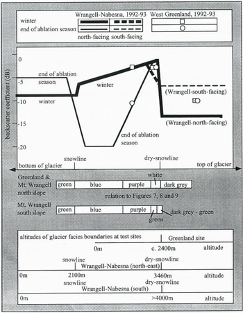
Fig. 13. Schematic and simplified illustration of SAR multi-temporal signatures for discrimination of glacier facies (applicable to ERS-1).
Confirmation is provided of the stability of the ERS-l (to 0.2 dB), using a natural, distributed calibration target. Both the Greenland dry-snow and percolation facies can be used as a natural calibration surface, as long as there is no surface melt.
Table 6. Summary of estimated altitudes of dry-snow line and snowline on Greenland (1992) and Mount Wrangell (1993)

Recommendation
In this paper, it is demonstrated that significant detail on the glacier facies can be provided from multi-temporal SAR image data. It is recommended that a multi-temporal (colour) SAR image mosaic of glacier facies across Greenland be generated using the techniques described in this paper. With continuous polar-orbiting SAR missions anticipated in the foreseeable future, it should be possible to generate such a mosaic on a repeated basis in order to monitor long-term movement of the glacier facies, albeit with superimposed short-term variations. The technique described here provides a graphic and sensitive means of detecting movement of the facies.
Acknowledgements
The anonymous referees and M. Sturm provided very useful comments. In addition, useful discussions were held with K. Ahlnaes, J. Bamber, C. Benson, K. Jezek, C. Lingle, G.
Marshall, M. Rast, H. Rott and A. J. Sephton. Thanks are also extended to H. Rott for providing the meteorological data and T. Logan for preparing the USGS DEM data. The Greenland data analysis was supported under contract 10063/92/NL/SF for the European Space Research and Technology Centre, Noordwijk, Netherlands to GEC-Marconi Research Centre. The Alaska data analysts and the paper preparation were carried out using the science tools available from the Alaska SAR Facility, Geophysical Institute, University of Alaska—Fairbanks (Website http:// HYPERLINK "http://www.asf.alaska.edu" www.asf.alaska.edu), with data provided by K. Ahlnaes and G. Lingle. All SAR data were made available by the ESA. Figure 1 is provided courtesy of C. Benson.


