


Introduction
Glaciers in Spitsbergen, Svalbard, are traditionally classified as sub-polar or polythermal in respect of their thermal structure (Reference SchyttSchytt, 1969; Reference BaranowskiBaranowski, 1977). They have a thick layer of cold ice (with temperatures below the pressure-melting point) in their superimposed-ice accumulation and ablation zones, usually underlain by temperate ice at the pressure-melting point, though they may be frozen to the bed in places. In the firn accumulation zone the whole thickness of the ice is temperate, with only the winter cold wave lowering the temperature of the near-surface firn below freezing. The large difference in the dielectric properties of ice and water makes radar sounding a useful tool for discriminating between ice containing water and ice that is dry, i.e. cold ice. An internal radar-reflection horizon in the ice may not correspond precisely with the pressure-melting-point isotherm in the glacier, due to the size of the water bodies relative to the radar wavelength (e.g. Reference Ødegård, Hagen and Hamran.Ødegård and others, 1997), or to the possibility of water bodies existing in cold ice. The general scheme of sub-polar glacier structure was confirmed by airborne radio-echo sounding (RES) by Soviet (Machert and Zhuravlev, 1982, 1985) and British-Norwegian groups (Reference Dowdeswell, Drewry, Liest$l and OrheimDowdeswell and others, 1984). One or other of the groups flew over the majority of glaciers in Svalbard. Ground-based radar soundings have provided a more detailed and complex picture of the thermal structure of some of these glaciers (e.g. Reference Björnsson.Björnsson and others, 1996; Reference Hamran, Aarholt, Hagen and Mo.Hamran and others, 1996; Reference Ødegård, Hagen and Hamran.Ødegård and others, 1997). In some cases, cold ice dominates and only the glacier sole is at the pressure-melting point. Traditionally, radar sounding of glaciers has been done using rather low-resolution radars (e.g. Reference Bogorodsky, Bentley and GudmandsenBogorodsky and others, 1985, ch.4). Recently, modern ground-penetrating radar (GPR) that can operate successfully on polythermal and temperate glaciers has become available (e.g. Reference Murray, Gooch and StuartMurray and others, 1997).
Temperate ice has been observed in the ablation zone of Hansbreen (Fig. 1), a grounded, tidewater glacier that flows into the fjord of Hornsund, southern Svalbard (Reference GrześGrześ, 1980; Reference Jania and PulinaJania and Pulina, 1990). Results of rather low-frequency 8 MHz centre frequency) radar sounding at several dozen discrete points on the glacier surface in April 1989 showed many places with internal reflection horizons (Reference Glazovskiy, Kolondra, Moskalevskiy and Yaniya.Glazovskiy and others, 1992; revised data in Reference KotlyakovKotlyakov, 1992, p.81). Based on detailed study of the velocity variation of radar waves with depth at one point on the glacier, Reference Macheret, Moskalevsky and Vasilenko.Macheret and others (1993) proposed a three-layer model for the glacier, with different water contents and températures for each layer. Reference Jania, Mochnacki and GadekJania and others (1996) presented ice-temperature measurements from several boreholes and interpreted the data from the previous RES in a four-layer model. Difficulties in reconciling the RES data with borehole-temperature measurements prompted the current investigation of the internal structure of the glacier by higher-frequency radar operating with much better spatial resolution than had been available earlier.

Fig. 1. Location map of Hansbreen. The 50 MHz profiles are solid lines numbered 1-4, and 200 MHz profiles are broken lines numbered 5-7. The locations of boreholes with thermistor chains are shown as open circles labeled D, F, G, H, I. The locations of the radargrams shown in Figures 2—4 are shown along with the site H5 of the low frequency radar common-depth-point site of Reference Macheret, Moskalevsky and Vasilenko.Macheret and others (1993). The 12 August 1990 snowline is shown on Hansbreen and Staszelisen, and the Firn-ice transition region from the GPR profiles (representing the 1997 firn line) is also marked on profiles 2, 4, 6and 7.
Our aim was to relate the internal structure from the radar sounding to the temperature data from the boreholes and study the distribution of cold ire in the glacier. In this paper we present comparisons of the radar internal reflection horizons observed at 50 MHz with the RAMAC GPR, with 1 m spacing between scans, and those from the earlier lower-frequency 8 MHz monopulse radar (Reference Macheret, Moskalevsky and Vasilenko.Macheret and others, 1993), at spot positions on the glacier. We also compare the observed radar reflection horizon with temperature profiles at four boreholes close to the radar profiles. We present high-resolution profiles of the cold ice layer and its contact with temperate ice, and use the radar to examine the influence of crevasses and moulins on I he thickness of the cold ice and the amount of water present in the ice.
Radar Sounding
In May 1997 we used a RAMAC GPR operating at 50 and 200 MHz to profile Hansbreen and some associated glaciers in Hornsund (Fig. 1). The technique involved driving the profile lines on a snowmobile carrying hand-held GPS receivers, followed by another snowmobile that pulled the radar behind it. The radar antennas were mounted on a non-metallic sledge separated by 5 m from the snowmobile. The radar control unit and computer were carried on the snowmobile and controlled by a passenger, leaving the driver free to follow the line prepared by the earlier GPS snowmobile. Data were collected on a Husky portable computer and stored on hard disk, which worked well even in temperatures below -30°C. The 50 MHz data were collected in the form of 2048 samples and a time window of 5.303 μs. The 200 MHz data were collected in the form of 1024 samples and a time window of 0.692 μs. Both 50 and 200 MHz data were stacked twice on collection. It was possible to use extra power from standard 12 V accumulators in addition to the RAMAC and computer battery packs to provide enough power for a full day of operation without recharging.
Data were collected at 1 m intervals with triggering from a sledge wheel mounted on the snowmobile. Position accuracy was maintained by passing close to several geodetically surveyed stakes on the glacier, and the sledge wheel was found to be surprisingly accurate for the 50 MHz data. Unfortunately, the readings for the 200 MHz lines that were taken later show large discrepancies, probably due to a faulty mechanical connection between the wheel axle and the electronic sensor. Problems were also encountered with GPS coordinates from hand-held Magellan and Garmin 45 receivers, with errors of up to 250 m. We believe that the 50 MHz radar profiles are always within 50-100 m of the positions plotted in Figure 1. However, the 200 MHz data cannot he located as accurately.
Radar interpretation methods
A variety of techniques can be used to interpret radar data in terms of the physical properties of the materials being investigated. One traditional technique is common-depth-point (CDP) sounding whereby the transmitter and receiver antennas are separated as the data are recorded. Geometric analysis then gives radar-wave velocities in discrete layers in the media (assuming the layering is nearly horizontal), and the radar velocities can then be converted to water contents in the ice ( Reference Macheret, Moskalevsky and Vasilenko.Macheret and others, 1993). This method, though accurate, is slow and cannot give wide coverage on the glacier. Another method is to use the back-scattering energy as a measure of the change in dielectric properties at a reflecting surface, and from that change to estimate the water content, providing a reasonable model of the water-scattering bodies can be found. Reference Hamran, Aarholt, Hagen and Mo.Hamran and others (1996) showed that this method can give good spatial coverage of water content on Svalbard glaciers assuming that the size distribution of the scattering particles is constant. The attenuation and scattering of radar waves as a function of scatterer size are essentially governed by Mie theory for circular scatterers. If the scatterers are not exactly spherical or if there is a dispersion in sizes, the rule of thumb is that for particles greater than a wavelength in circumference, the scattering efficiency is unity, while for smaller scatterers the efficiency falls off as wavelength to the fourth power. In other words, for a single scatterer smaller than a wavelength, an increase in wavelength by a factor of 2 decreases the scattering efficiency by a factor of 16. Note that this holds only for scattering efficiency, while the scattering cross-section is found by multiplying the efficiency by the number density of the scattering centers. This is not known for real glaciers, but in most natural systems there is a power-law dependence on size for the number density. If that law has exponent 3, then the backscatter is dominated by particles near a wavelength in size, hence the usual radar assertion that we mainly measure particles the size of the wavelength. If the power-law exponent is 4, then cross-section is dominated by the small particles, but if the exponent is 2, the large ones govern.
In this paper we use a different method to measure water content, based on the travel time to point-scattering centres that can be seen individually in the radar data. In practice, this means that the scattering objects are smaller than the resolving power of the antennas; in the case of 50 MHz this means below about 2 m in any dimension. If scattering objects are elongated in one direction (such as a buried crevasse), simple scattering as assumed here will not be valid. As the antennas approach a point object the radar waves will travel through different ice thicknesses, and the return seen on a radar profile such as Figure 2 will be a hyperbola, with opening angle dependent on the radar velocity, and hence water content of the ice. Removal of these hyperbolas is the basis of the migration procedure commonly used in seismic processing, and has also been used with radar data on glaciers (e.g.Reference Welch, Pfeffer, Harper and HumphreyWelch and others, 1998). Here we use the hyperbola to give information on the radar-velocity variations in the ice. Scattering bodies at different depths can be used to produce a depth-varying model of velocity. Though the ice need not have uniform radar velocity as a function of depth, any lateral variability cannot be resolved and will appear as distortions in the hyperbolic shape.

Fig. 2. A typical section of 50 MHzGPR data from the western end of profile 1. The character of the reflections is typical offirn at 6000-6500 m.Warm ice associated with much scattering, and cold ice associated with down-dipping foliations from 5750 m to the intersection with the warm ice at 6050 m, can be seen. A large hyperbolic reflection at 5800 m at 85 m depth is probably a water channel or pocket. A series of sharp hyperbolic reflections near the surface at 6500 m are probably caused by crevasses associated with the bedrock bump and the change in surface slope.
If the velocity of the penetrating radar wave is v, the relative dielectric constant εr of the media can be calculated as

where c is the velocity of light. When the depth of the point reflector is known, the velocity is:

where T1, T2 are the one-way travel times to the reflector for two points on the surface with separation x, and z is depth of the reflector. If T1 is measured on top of the reflector, so that it is the shortest travel time to the reflector, T0, the depth of the reflector is:

From Equation (3), the average velocity of the electromagnetic wave between the glacier surface and the point reflector is:

The distance x must be measured as accurately as possible, and it is assumed that the transmitter and receiver antennas have zero separation. In the GPR system used here, however, the antenna separation was 2 m for 50 MHz, and 0.6 m for 200 MHz. This causes an error which quickly becomes negligible with depth. The velocity found is the average for the ice between the reflector and the antenna. It is possible to assign separate velocities to various layers within the ice, so that the velocity in the layer of interest can be found. Thus, if a layer of dry, cold ice overlays wet ice, the boundary between the layers can be found and the cold ice assigned a velocity corresponding to a solid-ice permitivity of 3.19. The Haescan radar interpretation program (RoadScanners, Rovaniemi, Finland) allows this to be done interactively, but refraction at the layer interfaces is not considered in the calculations.
The average relative permittivity in the layer of interest can be converted to the water content of the ice using dielectric mixture relations. Reference Macheret, Moskalevsky and Vasilenko.Macheret and others (1993) used Paren's mixture formula to produce an expression that can be rewritten as:
where W is the water content, εr is the permittivity of the ice above the hyperbola, εi is the permittivity of solid dry ice (taken as 3.19) and εw is the permittivity of water (taken as 86). However, Reference Frolov and Macheret.Frolov and Macheret (1998) further considered the relation between ice with a density-dependent permittivity εd, water content and radar-wave velocity to derive a more complete relationship using the Looyenga mixing formula:

The large-scale bulk density of glacier ice is probably less than that of solid monolithic ice since the ice will have some fraction that is occupied by channels, inclusions, voids, etc. Densities from ice cores on Svalbard (Reference Frolov and Macheret.Frolov and Macheret,1998) indicate bulk densities of > 908 kg m -3, which corresponds to a permittivity εd of about 3.16. This is so close to the value of εi that we consider density effects to be negligible in the calculation of W. A convenient and accurate way of calculating W is to use the least-squares second-order polynomial fit to permittivity change for 0.001 <W< 0.1:
There are differences between the values of W obtained from Equations (7) and (5) of up to 0.5% in absolute water content (Table 1).
Table 1. Calculated water contents for selected parts of the GPR profiles and the earlier 8 MHz RES CDP point, H5

Since water has a relative permittivity of 86 and that of solid ice is around 3.2, the permittivity of an ice/water mixture (and hence radar velocity) is very sensitive to water content. The errors associated with the hyperbola-fitting method for estimating water contents are individually quite high. However, because so many hyperbolic reflection patterns are present, and assuming the individual errors are independent, which seems likely, it is possible to obtain statistically meaningful results.
The phase change on reflection of radar waves from a contact between media with different dielectric constants has been used as an aid to interpretation of radar data (Reference Arcone, Lawson and DelaneyArcone and others, 1995). Such a technique would be of great value in determining if a cavity in ice was water or air filled, but distortions in wavelet shape as the radar wave passes through the many dielectric contrasts in firn and ice make this technique unusable in our experience. A similar conclusion can be drawn from modelling studies with ice cores (Reference Kohler., Moore, Kennett, Engeset and ElvehØy.Kohler and others, 1997; Reference Miners, Blindow and GerlandMiners and others, 1998). However, the reflection coefficient will be much greater at a water-filled cavity than from a rock or air void of similar dimensions, due to the much greater dielectric contrast between ice and water than between ice and air or rock. Unfortunately, as the backscatter also depends on the object's size, we cannot unequivocally determine the nature of the object causing the scattering. We assume that point scatterers are most likely to be water bodies if they are very bright objects. Also Hansbreen has well-defined moraines, with few rocks visible in the ablation zones away from these moraines.
Many of the features generally seen in the GPR images are shown in Figure 2, particularly the bedrock reflection, a clear hyperbolic reflection probably from a water channel in the ice, the differing characters of reflections from cold and warm ice and firn, and a near-surface crevasse. As we are primarily interested in deep reflectors, radar travel times were converted to depths using a permittivity value of 3.19 corresponding to a radar-wave velocity of 168 mμs-1. In the firn area, one small correction should be made to allow for the lower-density surface layers, and another of opposite sign to account for water present in the temperate ice. Since these corrections are likely to be fairly small and in the opposite direction over much of the glacier, we neglect them in the profiles we present. Although water-saturated areas can cause a significant decrease in velocity and corresponding overestimation of the depth of ice, Reference Macheret, Moskalevsky and Vasilenko.Macheret and others (1993) find radar-wave velocities close to the value we use for Hansbreen. The 200 MHz data were used mainly for studies of the snow and surface layers and we used a characteristic velocity of 220 m μs-1 . Depth resolution is limited by the radar pulselength (1/bandwidth). In a monopulse GPR system such as used here, the resolution is about 2 m in ice at 50 MHz, and about 1m in snow at 200 MHz. Depth penetration is attenuation- and clutter-limited to about 350m with 50 MHz antennas. The time window defined for the 200 MHz antennas limited depth penetration to about 50 m.
Hydrology of Hansbreen
Reference Jania, Pulina, Sand. and KillingtveitJania and Pulina (1994) discuss the hydrology of several glaciers in southern Svalbard, including Hansbreen, in some detail. Almost the whole basin containing Hansbreen is drained by subglacial channels, and melt water flows directly to the sea. During summer, two or three outflows of turbid fresh water from the frontal ice cliffs are typically observed. The glacial drainage system has been mapped in the field and from aerial photographs taken in 1990. Water flow through cold ice may be associated with moulins, crevasses or other channels within the ice. On Hansbreen the moulins usually form in local depressions associated with crevasses, foliations or shear lines. Twelve moulins on Hansbreen were investigated by Reference Schroeder and GriselinSchroeder (1995). The moulins are located in zones associated with the bedrock sills of overdeepened basins as determined by the RES of Reference Glazovskiy, Kolondra, Moskalevskiy and Yaniya.Glazovskiy and others (1992). Only two of the moulins are near the radar profiles, including the most important moulin system, Basa Cave (Fig. 1), which drains about 3.8km2 of the glacier surface and conducted about 6 to 7× 10⁶ m3 of water in 1990 and 1991 (Reference Jania, Pulina, Sand. and KillingtveitJania and Pulina, 1994). Baza Cave and M31 are located on profile 4 (Fig. 1), and the radar profile near Baza Cave is shown in Figure 3. Water depths were measured in September 1991 and May 1992 and are shown in Table 2 along with data for other moulins on the glacier.
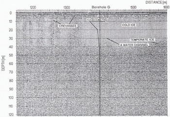
Fig. 3. GPR section of 50 MHz data from profile 4 around borehole G. A crevasse zone exists down-glacier of borehole G and is marked by sharp hyperbolic reflections between 1200 and 1320 m. The warm ice beneath this zone appears to have higher water content ( Table 1) than the ice up-glacier of the borehole which is not in a crevasse zone. The temperature profile from the borehole is shown on the image, with measurements at 10 m intervals. The pressure-melting point coincides closely with the change in character of the GPR reflections around 40 m depth.
Table 2. Depth of water in several moulins on Hansbreen (after Reference Schroeder and GriselinSchroeder, 1995)

The pattern of water flow in the temperate parts of the glacier can be inferred from observations during Russian ice-core drilling in the temperate accumulation area of Amundsenisen, southern Spitsbergen. Micro-channels have been found at several levels below 150 m (Reference Zagorodnov and ZotikovZagorodnov and Zotikov, 1981). They form horizontal fissures, vertical, semicircular channels 4-8mm2 in cross-section and small tubes parallel to the glacier surface about 100 mm2 in cross-section filled with highly mineralized water (personal communication from M. Pulina, 1998). Similar micro-channels were present in the drillhole in the accumulation zone of Fridtjovbreen, western Spitsbergen, at depths of about 100 m (Reference Zagorodnov and KotlyakovZagorodnov, 1985). Similar features may be present in other Spitsbergen glaciers, including Hansbreen. Chemical analysis of the surface layers of Hansbreen shows that the winter snow contains 5-10 times the salt content of deeper layers (Reference Jania, Mochnacki and GadekJania and others, 1996). Though some salts are carried off the glacier in surface melt streams, much of the salt migrates downwards in the firn area with percolating water (Reference Glowacki and Glowacki.Glowacki, 1997). The mineralization of water in channels within the glacier is eight times higher than found in percolating water (Reference Glowacki and Glowacki.Glowacki, 1997). This higher-salinity water will lower the freezing point and allow effective transmission of the latent heat of fusion through the liquid into the deeper firn areas.
Thermal Structure of Hansbreen
Borehole thermometry and GPR
A series of boreholes, marked in Figure 1, instrumented with thermistors has been drilled on Hansbreen (Reference Jania, Mochnacki and GadekJania and others, 1996). GPR data were unfortunately only collected directly next to boreholes F and G (Fig. 3). The only data on ice temperatures to compare with the GPR data on the cold/ warm ice transition come from G (borehole F indicating temperate ice throughout the glacier). Temperatures were measured at 10 m intervals starting 20 m below the surface, so resolution of the cold/warm ice boundary is limited. However, Figure 3 shows that the boundary is consistent with the change from ice with little scattering to ice with much scattering of radar waves. The surface markers for the other boreholes were not visible above the winter snow layer present during the GPR survey, and therefore only profiles close to their estimated positions could be made. Borehole H shows about 70 m of cold ice, which is consistent with the area closest to it on profile 4 (about 150 m east of the borehole), where there is about 60 m of cold ice. Borehole D was located about 150 m up-glacier from profile 2, and the temperature profile indicated about 70 m of cold ice. However, the region of profile 2 near borehole D shows only 40 m of cold ice. Since the radar profile is down-glacier of the borehole we would have expected there to be more cold ice present than higher up the glacier as is seen in profile 4, though there may be some advection of cold ice from tributary-glaciers to the cast of Hansbreen. We cannot explain this discrepancy in cold-ice thickness from the limited observations we have in the area; 200 MHz profiles 5-7 did not penetrate deep enough to give data on the cold-ice thickness.
The transition condition at the cold/temperate transition surface (CTS) is

where κ is the thermal conductivity of ice (2.1 W K-1 m-1), ρ is the density (910 kg m-3), L is the specific heat of fusion (3.5 x 10 -5 J kg-1 and W are the temperature and the water content on the cold and temperate side of the CTS, respectively, u is the velocity of the CTS, v is the velocity of the ice at the CTS and n is the unit-normal vector of the CTS pointing to the cold side. The righthand side of Equation (8), anW, is the freezing rate, with n the normal component of the velocity of the ice relative to the (also moving) phase boundary times the unit area; thus it is the normal volume flux. The dominant vertical component of the temperature gradient, ∂θ/∂z, can be measured in boreholes. W can be estimated by the method presented earlier and n can be determined from radar maps of the CTS.
At borehole G (Fig. 3), assuming that the borehole is located in the drier ice region where water contents are 1.2% (Table 1), and taking the temperature gradient in the cold ice to be about 0.03° C m-1 (Reference Jania, Mochnacki and GadekJania and others, 1996; Fig. 3), we obtain a freezing rate of 0.5 ma-1 or, if the borehole is in the wetter ice, 0.15 m a-1. This is comparable to the Freezing rates calculated by Reference Ødegård, Hagen and Hamran.Ødegård and others (1997) for Finsterwalderbreen in the superimposed-ice accumulation zone and ablation zone.
The temperature measurements from borehole G do not give enough information to determine an or even the velocities u and v separately.
The thickness of the cold ice along profile 4 is shown in Figure 4. A consistent thinning of the cold ice layer down-glacier of the firn and supposed superimposed zone cannot be seen in Figure 4, probably because of the influence of lateral glacier flow into Hansbreen and possible departures of GPR profile 4 from a flowline. Also shown in Figure 4 is a comparison of the cold, dry/temperate ice interface and the borehole thermometry and water-level depths in moulins near the profile. We can see that the depths of the cold ice layer at M31 and Basa Cave agree quite well with the water levels, though the differences in water level are large even over a few days (Table 2). We would expect that the position of the water table as observed from moulins should correspond closely with the depth of the upper boundary of the radar returns that we associate with scattering from water inclusions in the ice. We would also expect that ice-temperature measurement by borehole thermometry would be rather less sensitive to rapid water-table fluctuations and would record a melting-point depth that corresponds to a longer-term average. However, the variations in water table suggest that detailed comparisons between depths of GPR reflectors, water level and borehole thermometry are prone to misinterpretation unless they are all performed around the same time. It is also noticeable that the thickness of the cold ice layer decreases across the moulin zones and associated bedrock sills. This could be a result of water inflow from the moulins or a change in ice flow as the glacier advances across the sills.

Fig. 4. Interpretation of profile 4 showing the internal structure of the longitudinal profile of Hansbreen, with the position of Baza Cave and the M31 moulin end boreholes F,G andH marked. The depth of the water table in the moulins from Table 1 is plotted as an "error bar" below the moulin. The bedrock could be seen only intermittently between 8853 and 13754 m, so we have used earlier RES data (Reference Glazovskiy, Kolondra, Moskalevskiy and Yaniya.Glazovskiy and others, 1992) to complete the profile.
There are occasional near-surface reflections that appear to originate as supraglacial rivers in the cold ice zone (e.g. Fig. 3; Table 1). The hyperbolic reflections at depth in the cold ice probably do not come from large boulders, as the reflection coefficients seem rather high. More likely they are produced by water/ice interfaces. The channels or inclusions in the cold ice probably represent discreet Röthlisberger channels in the glacier ice. The size of these channels is unknown, as they appear to be point scatterers at 50 MHz, corresponding to a maximum size of a few meters. If we take the temperature gradient in the cold ice to be about 0.03°Cm-1 (Reference Jania, Mochnacki and GadekJania and others, 1996; Fig. 3) and assuming ice thermal properties as before, then channels of meter dimensions would remain open for many years even without any water flow, especially if the water is highly mineralized and so of lower freezing point than the ice surrounding it. The stability of the channels is thus probably very long-term.
Comparison with earlier RES on Hansbreen
The previous soundings using 8 MHz center frequency radar (Reference Glazovskiy, Kolondra, Moskalevskiy and Yaniya.Glazovskiy and others, 1992; Reference Macheret, Moskalevsky and Vasilenko.Macheret and others, 1993) were made at many discrete positions on the glacier, several of which were near to the GPR profiles measured in 1997. The equipment used was able to detect the bedrock echo all over Hansbreen; recording was by photographing an oscilloscope trace connected to the receiver. A CDP survey was conducted near the middle of the glacier at point H5 (Fig. 1) and was used as the basis of several hydrothermal models of the glacier (Reference Macheret, Moskalevsky and Vasilenko.Macheret and others, 1993; Reference Jania, Mochnacki and GadekJania and others, 1996).
The ice depths at the locations of the low-frequency RES (Reference Glazovskiy, Kolondra, Moskalevskiy and Yaniya.Glazovskiy and others, 1992) are in general agreement with our GPR data, though the GPR depths tend to be shallower by about 30 m. However, these data are difficult to compare closely because of uncertainties in relative locations of the radar survey positions, and the variability in the glacier surface between surveys, which could amount to 10 m or so in the ablation area (Reference Jania, Glowacki and KrawczykJania and Glowacki, 1996). The analogue recording by photography of an oscilloscope screen could lead to errors for the low-frequency data of about 3 m (personal communication from Yu.Ya. Macheret, 1998), due to factors such as the relatively low contrast range of the photographic film, the large spot size and the limited dynamic range of the oscilloscope. The digital GPR data are band-width-limited in resolution, which corresponds to about 2 m at 50 MHz.
The only place with evidence for larger discrepancies in ice thickness is the region near to Kvitungisen at the northeastern end of profile 3 (Fig. 1). lce thicknesses measured in 1997 are about 40-60 m lower than the earlier values, though there are only a few points where our data are close enough for direct comparison with those of Reference Glazovskiy, Kolondra, Moskalevskiy and Yaniya.Glazovskiy and others (1992). This large difference in ice thickness may be due to a surge that occurred in 1994-95 (personal communication from P. Glowacki and J. Rodzik, 1998), of Paierlbreen, the glacier to the east of Hansbreen.The surge has resulted in thinning of ice in the upper glacier basins feeding it, including Kvitungisen and the ice divide between it and Hansbreen(Fig. 1).
It is of interest to compare the depths of the hydrothermal boundary detected by the radars at quite different frequencies. Reflections may appear to come from different depths for two different frequencies as a result of the change in size of scattering bodies relative to radar wavelength, as was observed by Reference Ødegård, Hagen and Hamran.Ødegård and others (1997) on Finsterwalderbreen. Several internal reflection horizons were detected in the low-frequency data (Reference Glazovskiy, Kolondra, Moskalevskiy and Yaniya.Glazovskiy and others, 1992; Reference Macheret, Moskalevsky and Vasilenko.Macheret and others, 1993), but the only data available are along the center line of Hansbreen, especially near to the CDP survey point H5 (Fig. 1). In general, two horizons were observed in the center profile, though from the examples of the oscilloscope traces given in Reference Macheret, Moskalevsky and Vasilenko.Macheret and others (1993), interpretation of the reflections is difficult. At the CDP site, however, the data were interpreted as showing an upper cold layer 127 m thick underlain by about 60 m of temperate ice with a radar velocity of 145 m μs-1 , corresponding to a water content of 4%, underlain by temperate ice with a water content of about 1%.
In comparison, the lm horizontally spaced GPR data show much lateral variability of the hydrothermal boundary that could not have been followed with the discrete sampling points of the earlier survey. From Table 1 it can be seen that we do find quite wet areas of temperate ice. The area around H5 (7500-8000 m along profile 4) shows an upper cold layer 60-80 m thick, underlain by about 250 m of temperate ice with water contents of 0.8%, 2.2%, 2.9% and 3.9% (values are from 7533, 7657, 8071 and 7812 m, respectively, of profile 4 in Table 1). This wet ice, in turn, is underlain by temperate ice with water contents of 0.8% and 1,5% (from 7505 and 7684 m, respectively), and at 7998 m the permittivity indicates essentially zero water content. Thus, we observe a cold surface layer, a wetter temperate layer and a deeper but drier layer, as was seen in the earlier CDP survey. There are, however, differences in layer thickness between the surveys, which is not unexpected considering the rapid lateral variations in the hydrothermal structure of the glacier visible in the GPR profiles.
Lateral variations in hydrothermal conditions
Table 1 shows the results of calculations of the water content, deduced from the hyperbolic reflection patterns, for the parts of the glacier represented in the figures in this paper. These are representative of the rest of the profiles (Reference PälliPälli, 1998). Generally, we observe an increase in water content of the temperate ice beneath surface crevasses (Fig. 3; Table 1), and (with less certainty) in regions where there are moulins. The observations of hyperbolic reflections from either channels, water inclusions or possibly boulders in the ice allow us to investigate the water content over quite short distances. The wetter parts of the glacier typically contain about 4% water, which is in good agreement with the wet layer of temperate ice found by Reference Macheret, Moskalevsky and Vasilenko.Macheret and others (1993) at H5 (Fig. 1). The presence of wetter ice beneath crevasse zones may be an obvious result of water draining along the glacier surface and passing down crevasses and moulins to the temperate ice below the cold ice. Figure 5 also exhibits a feature which is probably a surface water channel filled with winter snow. Table 1 shows that there is also a high water content associated with this feature, which is consistent with this interpretation.

Fig. 5. The firn-ice transition in 50 MHz GPR data from profile 4. Approximately the top 20 m of firn, extending up-glacier from around 9100 m, shows fairly horizontal layering with spacing around 2 m which may represent annual layering of snow accumulation. At greater depths the layering is no longer visible, and general scattering from many refeclors characterizes the warm ice. The cold ice is a wedge shape having warm ice both beneath and on top of it. Foliations dipping down towards the firn can be seen in the cold ice. A multiple reflector at 9060 m coming from near the surface may be a strong reflection from a supraglacial river channel filled with winter snow.
Foliations
Foliations are defined as planar or layered structures that develop in glacier ice during flow; layers are characterized by variations in crystal size and air-bubble content (Paterson, 1994, p. 174). The weak radar reflections seen in cold, dry ice must arise from variations in the dielectric properties of the ice due to changes in air-bubble content (density), impurity concentration or preferred crystallographic orientation (Reference Bogorodsky, Bentley and GudmandsenBogorodsky and others, 1985, p. 164). Since foliations dip upwards in the ablation zone, as do the observed radar reflections, it seems reasonable to call these weak reflections radar foliations. Radar foliations in the ice that appear to follow bedrock topography are easily seen in most of the cold ice. The only exception is that there appear to be no foliations in the cold ice near the glacier terminus, where a zone of chaotic crevassing is associated with wet ice near the surface. The crevasses, or the warm ice, destroy the foliation generally preserved in the cold ice. Since there are places higher in the glacier where warm ice is present at the surface downstream of cold ice, we suppose that it is the particular ice flow associated with the crevassing and steeply rising bedrock that destroys the layering. Presumably the foliations are caused by the contrasts between bubbly-ice and solid-ice lenses and represent a weaker version (due to much less density contrast being possible in the impermeable ice) of the strong layering seen in the firn area.
Firn-ice transition
The firn line, unlike the equilibrium line, is a physically recognizable position on a glacier surface. On many glaciers both are in similar positions, but this is not the case on poly-thermal glaciers where superimposed ice represents a significant component of glacier mass balance. However, the firn line on glaciers such as Hansbreen marks the position of the occurrence of cold ice at the glacier surface (or to be more precise, beneath the winter snow cover).The physical nature of the transition from water-permeable firn to impermeable and cold ice is normally described (e.g. Reference MüllerMüller, 1962) as follows: the snowpack in the upper firn part of the glacier becomes wet with meltwater in the summer which then partly refreezes in lower layers, efficiently raising the temperature of the firn to the melting point. However, in lower regions the ice becomes impermeable to water, preventing penetration of meltwater except via crevasses or moulins. The ice is then cooled to below the melting point by heat loss in the long, cold winter period. The temperate cold transition in the near-surface layers probably does not coincide with the firn ice transition on the surface. Reference MüllerMüller (1962) divides firn into dry, upper and lower percolation zones. The transition between firn and ice is a complex zone starting in the lower percolation (soaked) zone and finishing in the superimposed-ice zone. The transition starts with the formation of ice lenses and ice layers in firn that contain much meltwater in summer. Some of this water refreezes, often after percolating along pipes to colder depths, and eventually spreads horizontally to form ice lenses. If the number of ice lenses grows, the permeability of the firn layers generally decreases and more water runs off. As a consequence, the heat released by refreezing drops and protects the deeper layers from becoming temperate in the summer.
The GPR image (Fig. 5) shows a section of the glacier where there is known to be firn from coring work. The firn is distinguished from ice by strongly layered reflections. This overlies cold, dry ice, which in turn is on top of ice with many hyperbolic reflectors, which we take to be scattering from water bodies within temperate ice. The layering in the firn is indicative of reflections coming from layers of markedly different dielectric constant, most probably through changes in density (Kollier and others, 1997). Winter snow accumulation in the vicinity of Figure 5 is 1.5-2 m (Reference Jania, Pulina, Sand. and KillingtveitJania and Pulina, 1994). The layers seen in the radar image are about 2 m apart (close to the limit of resolution of the 50 MHz radar), so it is likely that the dielectric contrasts causing them are from layers of ice lenses and relatively low-density firn. The thickness of the firn layer decreases gradually down-glacier to the point where only the winter snow cover is on top of uniform cold ice. The decrease in thickness of the layering downstream indicates that density contrasts are destroyed towards the firn-ice transition. which is consistent with the gradual increase in numbers of ice lenses in the lower percolation zone.
A stereo pair of aerial infrared false colour photographs were taken on 12 August 1990 (Norwegian Polar Institute Nos. 4055-4059). The photographs shows a clear line on the glacier between featureless white snow and parts with surface features such as crevasses. We have marked the position of this 1990 summer snowline in Figure 1. The summer ablation in 1989/90 was 0.77 m w.e, compared with an average (1988-94) of 0.52m w.e., the equilibrium-line altitude (ELA) was 380 m (32 m higher than average) and the mass balance was very negative over the whole glacier (Reference Glowacki and Glowacki.Glowacki, 1997, and personal communication 1998). It is clearly noticeable that the summer snowline extends almost north south down the central part of Hansbreen and also can be traced around Staszelisen. The trend of the line is similar to the pattern of snow accumulation and the trend of the ELA on Hansbreen, where more snow accumulates on the western side of the glacier than on the east (Reference Jania, Pulina, Sand. and KillingtveitJania and Pulina, 1994). We have marked the approximate position of the surface expression of the firn ice transition in Figure 1. Profile 4 intersects the 1990 summer snowline around scan 9400 (Fig. 4). It appears that the current firn region extends down-glacier of this by about 300-400 m. From Figure 4 it can be seen that the 32 m-above-average 1990 ELA corresponds to an up-glacier displacement of the ELA at profile 4 of about 1.2 km, whereas we observe a possible difference of only 400 m. However the close to parallel orientation of profile 4 and the ELA makes such comparisons difficult. The 1990 summer snowline on Staszelisen is crossed by profile 2 about 500 m from the start of the profile, very near the apparent firn line on the GPR profile (an analogous point in Figure 4 would be at scan 9100). The 200 MHz profiles 5 and 7 show similar features, but profile 6 shows a prolonged firn-ice transition, probably due to the profile running almost parallel to the firn line.
It is clear that the aerial photography from August 1990 does not indicate the same boundary on the glacier that we observe in the GPR data and interpret to be the firn line. However, the high degree of melting during the summer of the aerial photography is consistent with the long-term firn line (which would be observed by GPR being further down-glacier than the snowline in the photograph.
Conclusions
Using a commercially available GPR at 50 MHz it is possible to observe, at high lateral and vertical resolution, structures associated with changes in the hydrothermal conditions on Hansbreen. The cold-ice-temperate-ice boundary coincides with the water table in moulins and the melting point found from borehole thermometry, though field studies indicate that large changes in water level can occur rather quickly. The cold layer along the center line of Hansbreen varies from a maximum thickness of about 100 m just below the firn line, generally thinning down-glacier to the terminus. The firn-ice transition was investigated at both 50 and 200 MHz in a series of profiles on Hansbreen and a tributary glacier. The firn line on Hansbreen runs almost longitudinally along the glacier, probably as a result of greater snow accumulation on the west side of the glacier than the east. The firn-ice transition is quite wide, and consistent with a decrease in density contrasts between firn layers until the solid, uniform ice of the superimposed zone is reached. A comparison with the summer snowline from aerial photography does not show a clear link between snowline and firn line as determined by the GPR, though a general north-south trend is common to both lines.
Comparison of the depths of the temperate-/cold-ice boundary and the bedrock depth is reasonably consistent with earlier low-frequency RES surveys on Hansbreen, except near a part of the glacier that has been influenced by a surge on a neighboring glacier. Using a method of determining radar velocity to point reflectors, we deduce water contents at many parts of the glacier with comparable results to an earlier conventional CDP radar survey. The high spatial density of the GPR measurements allows the high variability in hydrothermal structure to be seen. Areas of wetter ice with water contents of about 4% seem to be associated with surface features such as moulins and crevasses which allow water to be fed to the temperate-ice aquifer beneath the cold-ice layer. In general, the temperate ice contains 1-2% water, but there are some regions that seem anomalous, some of which may be buried, partly frozen river channels or water-filled near-surface crevasses. There appear to be isolated water bodies or channels in the cold ice, which are probably of meter dimensions as they are easily visible in the radar images. Taking into account temperature gradients in the cold ice, the water inclusions may survive for many years, and are probably related to the stable large-scale drainage of the glacier. Freezing rates at the base of the cold ice are about 0.1 -0.5 m of ice per year.
Acknowledgements
Financial support came from the Finnish Academy grant No. 51854 and the Thule Institute supporting radar development. We thank the Polish Polar Station in Hornsund and the Norwegian Polar Institute for logistic support. The Polish group contribution was supported by the State Committee on Scientific Research (KBN) under the terms of grant No. 6-P04E-016-10 (to J.J.). Yu. Macheret provided much helpful guidance concerning the Russian literature.


