


INTRODUCTION
The modern climate of the Mediterranean region is influenced by high-pressure systems in summer and westerly storm tracks in winter, giving rise to a highly seasonal climate with dry summers, relatively wet winters, and strong seasonal temperature contrasts. Nevertheless, the climate of the region is not homogeneous and the pattern of climate changes across the region is complex (Lionello, Reference Lionello2012). There is a contrast between the reduction in annual precipitation during recent decades (1975–2015) across the Iberian Peninsula and in northern Italy, for example, and the generally positive trends in precipitation in Greece, the Balkans, and Turkey (Deitch et al., Reference Deitch, Sapundjieff and Feirer2017). This east-west dipole is also characteristic of rainfall trends over the twentieth century (Zittis, Reference Zittis2018) and during the Holocene (Peyron et al., Reference Peyron, Combourieu-Nebout, Brayshaw, Goring, Andrieu-Ponel, Desprat and Fletcher2017). It is highly likely that climate changes on longer timescales, specifically orbital timescales in response to change in insolation, and on glacial-interglacial timescales in response to changes in ice-sheet volume (Magri and Tzedakis, Reference Magri and Tzedakis2000; Rohling et al., Reference Rohling, Grant, Roberts and Larrasoaña2013), are equally complex.
The El Cañizar de Villarquemado palaeolake is located in Teruel province in the semi-arid interior of the Iberian Peninsula (40.49°N, 1.29°W, 985 m a.s.l.), and provides a pollen record that stretches from the end of the penultimate glacial (Marine Isotope Stage 6, MIS 6) through the last interglacial (MIS 5), the last glaciation (MIS 4–2), and into MIS 1 and the Holocene (Valero-Garcés et al., Reference Valero-Garcés, González-Sampériz, Gil-Romera, Benito, Moreno, Oliva-Urcia and Aranbarri2019; González-Sampériz et al., Reference González-Sampériz, Gil-Romera, García-Prieto, Aranbarri, Moreno, Morellón and Sevilla-Callejo2020). The length of the record and the quality of the age model make El Cañizar de Villarquemado an important site for documenting climate changes in the western Mediterranean, on both orbital (reflecting changes in precession, obliquity, and eccentricity on insolation) and glacial-interglacial (reflecting ice sheet and CO2 changes) timescales. The only other record from the western Mediterranean that spans this length of time is Padul (Pons and Reille, Reference Pons and Reille1988; Camuera et al., Reference Camuera, Jiménez-Moreno, Ramos-Román, García-Alix, Toney, Anderson and Jiménez-Espejo2018, Reference Camuera, Jiménez-Moreno, Ramos-Román, García-Alix, Toney, Anderson and Jiménez-Espejo2019), in southern Spain. Despite some similarities between the Padul and El Cañizar de Villarquemado pollen records, there are distinctive features that reflect their different climatic settings and sensitivities. There are also notable differences between the pollen record from El Cañizar de Villarquemado and other long records from the Mediterranean region, including the classic site of Tenaghi Phillippon in Greece (Tzedakis et al., Reference Tzedakis, Hooghiemstra and Palike2006; Milner et al., Reference Milner, Müller, Roucoux, Collier, Pross, Kalaitzidis, Christanis and Tzedakis2013), Lago di Monticchio in central Italy (Allen et al., Reference Allen, Watts and Huntley2000; Allen and Huntley, Reference Allen and Huntley2009, Reference Allen and Huntley2018; Martín-Puertas et al., Reference Martín-Puertas, Brauer, Wulf, Ott, Lauterbach and Dulski2014), and Lake Ohrid on the North Macedonia/Albania border (Wagner et al., Reference Wagner, Wilke, Francke, Albrecht, Baumgarten, Bertini and Combourieu-Nebout2017; Sinopoli et al., Reference Sinopoli, Masi, Regattieri, Wagner, Francke, Peyron and Sadori2018, Reference Sinopoli, Peyron, Masi, Holtvoeth, Francke, Wagner and Sadori2019), which suggest regional differentiation of long-term climate changes across the Mediterranean.
Inference of changes in precipitation from these long pollen records is complicated by large changes in atmospheric CO2 concentration [CO2] on glacial-interglacial timescales. [CO2] directly affects photosynthesis and water use (Ehleringer et al., Reference Ehleringer, Cerling and Helliker1997; Farquhar, Reference Farquhar1997; Prentice and Harrison, Reference Prentice and Harrison2009). Increasing [CO2] allows plants that use the standard C3 pathway of photosynthesis (including temperate grasses and forbs, and nearly all shrubs and trees) to assimilate more carbon while losing less water, implying an increase in water-use efficiency (Bramley et al., Reference Bramley, Turner, Siddique and Kole2013). Conversely, at low [CO2], C3 plants assimilate less carbon per unit water supply, necessarily resulting in reduced tree cover and a shift towards more drought-tolerant plants (including C4 plants). Shifts in the balance of steppe plants and tree taxa have been interpreted in terms of moisture-related climate variables (e.g., Sinopoli et al., Reference Sinopoli, Masi, Regattieri, Wagner, Francke, Peyron and Sadori2018; Camuera et al., Reference Camuera, Jiménez-Moreno, Ramos-Román, García-Alix, Toney, Anderson and Jiménez-Espejo2019), but this neglects the negative influence of low [CO2] on water-use efficiency. As a result, inferred or statistically reconstructed moisture variables are expected to indicate drier conditions than actually occurred (Prentice et al., Reference Prentice, Cleator, Huang, Harrison and Roulstone2017).
In this paper, we present a quantitative reconstruction of three bioclimatic variables: winter temperature (mean temperature of the coldest month, MTCO), growing-season warmth (growing degree days above a base level of 0°C, GDD0), and a moisture index (the ratio of annual precipitation to annual potential evapotranspiration, MI) using the pollen record from El Cañizar de Villarquemado and Tolerance-Weighted Averaging Partial Least Squares regression (TWA-PLS) (Liu et al., Reference Liu, Prentice, ter Braak and Harrison2020) that are calibrated using modern pollen (Harrison, Reference Harrison2019) and climate (Harrison, Reference Harrison2020) datasets for Europe and northern Eurasia. These three variables were chosen to represent the independent influences of extreme winter cold, integrated summer warmth, and plant-available moisture on the success of different plants. We apply a method of correcting MI to take account of the direct physiological influence of [CO2] on water-use efficiency. Although El Cañizar de Villarquemado is well dated, there are several intervals with poor pollen preservation, so we focus on the long-term evolution of climate rather than on abrupt climate changes. Finally, we compare our reconstructions with pollen-based reconstructions from the wider Mediterranean region.
METHODS
Modern Pollen and Climate Data
The modern pollen dataset, SPECIAL Modern Pollen Data Set (SMPDS), consists of relative abundance records of the 247 most important pollen taxa from 6458 terrestrial sites from Europe and northern Eurasia (Harrison, Reference Harrison2019; Turner et al., Reference Turner, Wei, Prentice and Harrison2020; Fig. 1). The SMPDS taxon list includes several layers of specificity: species, genera, sub-families, and families. Some taxa are represented at <10 sites and are therefore unlikely to provide a reliable basis for climate reconstructions. We used the 195 taxa that occur >10 times in the SMPDS as the initial basis for the climate reconstructions (Supplementary Table 1). We ran additional analyses after removing two taxa (Poaceae, Polypodiales) that displayed anomalous peaks in abundance that appeared to be related to changes in the sedimentary environment rather than climate. The final climate reconstructions are therefore based on 193 taxa.

Figure 1. Map showing the location of El Cañizar de Villarquemado and the distribution of modern pollen samples used in the calibration. The background map shows the climatological (1961–1990) mean temperature of the coldest month (MTCO, °C). Modern pollen data from Harrison (Reference Harrison2019) and modern climate data from the CRU CL 2.0 gridded dataset (New et al., Reference New, Lister, Hulme and Makin2002).
The modern climate at each of the SMPDS pollen sites was taken from Harrison (Reference Harrison2020). This dataset provides three bioclimatic variables: (a) mean temperature of the coldest month (MTCO), (b) growing degree days above a baseline of 0°C (GDD0), and (c) moisture index (MI). MI is the ratio of annual precipitation to annual potential evapotranspiration, calculated using climatological data (mean monthly temperature, precipitation, and fractional sunshine hours) derived from the CRU CL 2.0 gridded dataset of modern (1961–1990) surface climate at 10 arc minute resolution (~18 km) (New et al., Reference New, Lister, Hulme and Makin2002) and geographically weighted regression (GWR) to correct for elevation differences between each pollen site and the centroid of the corresponding grid cell. MI values were square-root transformed before analysis to emphasize the stronger vegetational differentiation at low MI.
Canonical correspondence analysis (CCA) (ter Braak, Reference ter Braak1986; Legendre and Legendre, Reference Legendre and Legendre2012) was used to perform a constrained ordination of the modern pollen data in response to the bioclimatic variables. CCA was implemented with the vegan package (Oksanen et al., Reference Oksanen, Blanchet, Friendly, Kindt, Legendre, McGlinn, Minchin, O'Hara, Simpson, Solymos, Stevens, Szoecs and Wagner2017) in R (v3.3.1). We examined the variance inflation factors (VIFs) to determine whether the predictors showed multi-collinearity. The significance of the CCA model was assessed with an ANOVA-like permutation test.
Fossil pollen data
The El Cañizar de Villarquemado palaeolake is located in the Jiloca basin in the semi-arid region of north-eastern Spain (Fig. 2). The site is occupied today by a wetland and cultivated land. The surrounding vegetation is dominated by evergreen or marcescent trees (e.g., Quercus ilex subsp. rotundifolia, Q. coccifera, Q. faginea) and xerophytic shrubs (e.g., Rhamnus lycioides, Genista scorpius, Ephedra fragilis, Thymus vulgaris, T. zygis). Juniperus (J. thurifera, J. phoenicea, J. communis, J. sabina, J. oxycedrus) and Pinus (P. sylvestris, P. pinaster, P. nigra) occur at higher elevations. The sequence provides a paleoenvironmental record spanning the interval from the last part of MIS 6 to the Late Holocene (Valero-Garcés et al., Reference Valero-Garcés, González-Sampériz, Gil-Romera, Benito, Moreno, Oliva-Urcia and Aranbarri2019; González-Sampériz et al., Reference González-Sampériz, Gil-Romera, García-Prieto, Aranbarri, Moreno, Morellón and Sevilla-Callejo2020). The age model from MIS 3 onwards is well constrained. Although uncertainties in the earlier part of the record are larger, the dates for key transitions in this part of the record are consistent with accepted estimates at the 90% confidence level (Valero-Garcés et al., Reference Valero-Garcés, González-Sampériz, Gil-Romera, Benito, Moreno, Oliva-Urcia and Aranbarri2019). Sedimentation rates are low during the initial part of the record and increase from the beginning of MIS 2 onwards. Intervals with poor pollen preservation occur between 16,000–22,300, 31,200–37,500, 43,100–50,100, and 87,900–93,800 cal yr BP. The average pollen sampling interval is ca 300 yr, increasing to ca. 140 yr during MIS 1. The pollen data were re-expressed in terms of the taxon groupings used in the modern pollen dataset for the application of TWA-PLS. The data used for TWA-PLS are available from http://dx.doi.org/10.17864/1947.219 (Harrison et al., Reference Harrison, González-Sampériz and Gil-Romera2019).

Figure 2. Vegetation map of El Cañizar de Villarquemado area showing dominant tree species, surface area of the basin and location of the core site.
TWA-PLS
The modern bioclimatic and pollen data were used to develop pollen-climate transfer functions independently for MTCO, GDD0, and √MI using tolerance-weighted-averaging partial least squares regression (TWA-PLS) (Liu et al., Reference Liu, Prentice, ter Braak and Harrison2020). TWA-PLS is an extension of weighted-averaging partial least squares regression (WA-PLS) (ter Braak and Juggins, Reference ter Braak and Juggins1993) that reduces the tendency of WA-PLS to produce climate reconstructions compressed towards the middle of the climate range represented by the modern training dataset. In TWA-PLS, taxon abundances are weighted by the inverse square of their modern climate tolerances. The theory behind TWA-PLS (a) assumes that the abundances of each taxon are unimodal with respect to the climate variable considered, and (b) follows a multinomial distribution. Under these conditions, TWA-PLS approximately minimises the difference between theoretical and actual abundances as assessed by the likelihood criterion. The performance of the calibration models was assessed through leave-one-out cross-validation. The number of components used in each model was estimated through a randomization t-test on the results of this cross-validation (van der Voet, Reference van der Voet1994). We selected the significant component with the lowest root mean square error of prediction (RMSEP), but only if there was a significant improvement in RMSEP relative to a lower number of components because including any more components results in over-fitting so that model predictive power decreases (ter Braak et al., Reference ter Braak, Juggins, Birks, van der Voet, Patil and Rao1993). We checked that the final transfer functions had a high R2 for prediction, and a low maximum bias.
We propagated the calibration errors into the down-core reconstructions by assessing the calibration error associated with each pollen sample using the “v1” option in rioja (Juggins, Reference Juggins2017). The errors arising from uncertainties in the modern pollen dataset tend to be large, so this approach emphasizes temporal differences in reconstruction uncertainty (results based on combining the two sets of uncertainties are shown in Supplementary Information).
Correcting for Changing [CO2] Concentration
Prentice et al. (Reference Prentice, Cleator, Huang, Harrison and Roulstone2017) developed a procedure to correct for direct effect of [CO2] on plant physiological processes. The procedure (Appendix 1) requires the specification of [CO2] and mean annual temperature (MAT). We used the ice-core [CO2] record (Bereiter et al., Reference Bereiter, Eggleston, Schmitt, Nehrbass-Ahles, Stocker, Fischer, Kipfstuhl and Chappellaz2015), smoothed using a LOESS smoothing spline with a span of 0.1. We estimated MAT for each site from the reconstructed MTCO and GDD0 at that site (Appendix 2). This calculation also allowed us to estimate the mean temperature of the warmest month (MTWA) (Appendix 2), which we then be used to generate a time series of temperature seasonality (MTWA−MTCO). We then converted the down-core reconstructions of √MI (and their maximum and minimum values) at El Cañizar de Villarquemado to MI, and applied the [CO2] correction to these MI values.
RESULTS
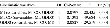
CCA showed a strong correlation between species abundance and the three climate variables in the modern pollen dataset, with correlations of 0.83, 0.61, and 0.47 respectively (Table 1). The VIF scores for each bioclimatic variable were low (<6), and the CCA indicates that they each have an independent contribution to explaining the variation in abundance. This was confirmed by the ANOVA-like permutation test, which showed that the bioclimatic variables and the three variability axes are all significantly different from one another (Table 1). As a further check, partial CCA was carried out using each predictor in turn (with the other two predictors as covariates). This confirmed that each predictor has a highly significant effect that it is independent of the others (Table 2).
Table 1. Summary statistics for the first three axes of CCA in the modern pollen dataset. The analysis was based on 6458 sites, 195 taxa, and three bioclimatic variables: mean temperature of the coldest month (MTCO, °C), growing degree days above 0°C (GDD0), and the moisture index (MI). Summary statistics for the ANOVA-like permutation test (999 permutations) are also shown.

Table 2. Summary statistics for the ANOVA-like permutation test (999 permutations) of partial CCA in the modern pollen dataset. Partial CCA analysis used each predictor in turn, with the other two predictors as covariates.
For TWA-PLS regression based on the full complement of 195 taxa, we used results from component 2 for MTCO and MI and component 1 for GDD0 because these are the significant results (95% confidence level) with the lowest RMSE and highest R2. The R2 values are 0.70, 0.66, and 0.52 for MTCO, GDD0, and √MI, respectively (Supplementary Table 2). Nevertheless, close examination of the down-core reconstructions revealed anomalous peaks in reconstructed MI, particularly at the end of MIS 5. These correspond to samples with unusually high values of either Poaceae or Polypodiales (Fig. 3), and where the sedimentary record indicates variability in environmental conditions and that the basin was occupied by wetlands. Under these conditions, the anomalously high peaks of Poaceae likely correspond to reeds, while the anomalously high peaks of Polypodiales probably represent inwash. Both Poaceae and Polypodiales were therefore removed from the final TWA-PLS model (Table 3), reducing the total number of taxa considered from 195 to 193. This alteration made no change to the number of components or the goodness-of-fit of the model (R2 values are 0.70, 0.68, and 0.51 for MTCO, GDD0, and √MI, respectively), but made the reconstructions of MI for the anomalous samples less extreme, more comparable to reconstructed values in adjacent samples, and therefore more plausible (Fig. 4). The removal of these taxa had no significant effect on the MTCO and GDD0 reconstructions (Supplementary Fig. 1). We checked whether particularly high or low values in the temperature reconstructions were a result of anomalous characteristics of the pollen assemblages, specifically whether there was evidence of pollen degradation (as measured by the fraction of indeterminable grains) or the samples were characterized by low biodiversity (as measured by the N2 index) (Hill, Reference Hill1973). There was no correlation between the abundance of indeterminable grains and anomalously high or low reconstruction values. However, depauperate samples tended to produce more extreme temperature values than adjacent more diverse samples (Supplementary Fig. 2). We therefore excluded samples with N2 <2 from the final reconstructions. Excluding samples with N2 <3 had little further effect on the reconstructions, but increased the patchiness of the reconstructions by removing a large number of samples.

Figure 3. Simplified stratigraphic and pollen diagram from El Cañizar de Villarquemado (a more complete diagram is given in González-Sampériz et al., Reference González-Sampériz, Gil-Romera, García-Prieto, Aranbarri, Moreno, Morellón and Sevilla-Callejo2020). The first column shows changes in inferred sedimentary environments, including the alternation between lacustrine and non-lacustrine conditions. The simplified pollen diagram shows the changing abundance of conifers, mesophyte trees, Mediterranean, and steppe taxa. We also show the changing abundance of aquatics and Polypodiales. The final column shows the biodiversity index (Hill's N2). The transitional phase at the beginning of MIS 5 corresponding to the Zeifen-Kattegat Oscillation is labelled Zeifen in the column showing the marine isotopic stages.

Figure 4. The impact of removing Poaceae and Polypodiales from the taxon set on reconstructions of moisture index (the ratio of annual precipitation to annual potential evapotranspiration, MI) during MIS 4 and MIS 5a. The reconstructed √MI has been re-expressed as MI, but no CO2 correction has been applied. The red line (without P/P) shows the values of MI once Poaceae and Polypodiales are removed. Removing these two taxa reduces anomalous peaks, where they were particularly abundant, but has little impact on the reconstructions for the rest of the core.
Table 3. Leave-one-out cross-validated predictions of the tolerance-weighted averaging partial least squares (WA-PLS) regression models used for the climate reconstructions. The P values were derived from a randomization t-test. The final model is based on 193 taxa, omitting Poaceae and Polypodiales. Selected components in the final model are marked in bold.

The final reconstructions (Fig. 5, Supplementary Tables 3, 4) show an increase in both summer (GDD0) and winter (MTCO) temperature between 130 and 127 ka. Both summer and winter temperature generally declined through MIS 5—although there are fluctuations, they do not correspond exactly with the chronological boundaries of sub-stages within MIS 5 (Fig. 5). Furthermore, the changes in summer and winter temperature are not in phase. Minimum winter temperatures occurred earlier than minimum summer temperature in MIS 5e, so that winter temperatures were already increasing while summer temperatures continued to decrease after ca. 120 ka. In contrast, during MIS 5a, warming in summer occurred around the same time as winter cooling, such that the temperature seasonality was significantly enhanced between ca. 80 and 70 ka. There was no pronounced cooling, either in summer or winter, at the transition into the glacial (Fig. 5). The record from both MIS 3 and MIS 2 is not continuous, and the available samples may show the response to millennial-scale events; thus, it is difficult to characterize the trends in temperature. However, MIS 3 appears to have been somewhat warmer than both MIS 2 and MIS 4 in summer (Supplementary Table 4). MIS 3 was not significantly warmer in winter than other intervals during the glacial, and there was a gradual decline in winter temperature from MIS 4 through MIS 3 to MIS 2 (Supplementary Tables 3, 4). MIS 1 was characterized by warming in both summer and winter, although the reconstructions show considerable variability superimposed on this trend.

Figure 5. Reconstructed mean temperature of the coldest month (MTCO, °C), growing degree days above a base level of 0°C (GDD0), and CO2 corrected moisture index (the ratio of annual precipitation to annual potential evapotranspiration, MI). The reconstructions are based on 193 taxa, after the removal of Poaceae and Polypodiales. Only samples with a Hill's N2 biodiversity index >2 are plotted. The marine isotope stages (MIS) and substages are shown by vertical dotted lines and labelled; we also show the transition interval between MIS 6 and MIS 5e. Red dots indicate the modern climate at the site. The error bars on the reconstructions, shown by shading around the mean value, are sample-specific errors (v1 in rioja).
The implied increase in temperature seasonality during MIS 5e, 5c, and 5a compared to during MIS 5d and 5b corresponds to the differences in seasonality in insolation between these stages (Fig. 6), primarily driven by summer insolation. Higher seasonality during the early part of MIS 1 also corresponds to increased seasonality in insolation compared to the present day (Fig. 6). Changes in seasonal differences in insolation across the glacial were muted. However, temperature seasonality was larger during MIS 3 and MIS 2 than during the interglacial intervals. Intervals of increased temperature seasonality during MIS 3 and MIS 2 cannot be explained by changes in the seasonality of insolation.

Figure 6. The correlation of the temperature seasonality and insolation. The black line in the top plot is the difference between reconstructed mean temperature of the coldest month and the mean temperature of the warmest month calculated based on MTCO and GDD0 (Appendix 2); we have applied a 1000 year time step with a span of 0.1 to draw attention to the major trends. The orange line in the top plot is the difference between July and January insolation in W m−2 at 40.49°N (the latitude of El Cañizar de Villarquemado). The bottom panel shows mid-monthly insolation anomalies (compared to present) in W m−2 at 40.49°N.
Conditions became progressively more humid from MIS 5e through to MIS 5c, while conditions were generally humid, but variable, during MIS 5a (Fig. 5, Supplementary Tables 3, 4). MIS 4 was also relatively humid, while MIS 3 was the most arid phase reconstructed during the glacial. However, the difference in reconstructed MI between MIS 4 or MIS 2 and MIS 3 is not large. This reflects the fact that [CO2] decreased throughout the glacial, so that the impact of the CO2 correction becomes larger from MIS 4 through MIS 3 and into MIS 2 (Fig. 7). The influence of changing [CO2] is most marked in dry climates (Fig. 8), which is why this effect has such an important influence on our reconstructions of MI. The highest values of MI are reconstructed during the deglaciation; there was a pronounced increase in aridity during the Holocene. The reconstructed changes in MI are anti-correlated with changes in GDD0 (r = −0.68), with decreased MI during intervals of summer warming. This suggests that the changes in MI may have been driven more by changes in evapotranspiration than by changes in precipitation.
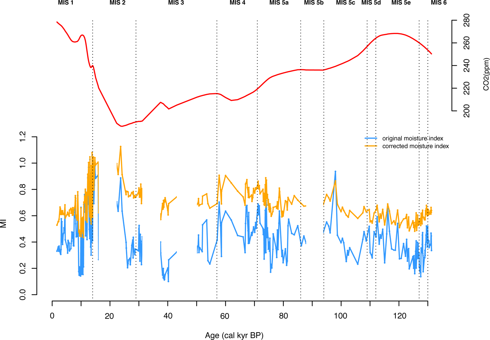
Figure 7. Changes in [CO2] and their impact on reconstructed moisture index (the ratio of annual precipitation to annual potential evapotranspiration, MI). The upper panel shows the changes in [CO2] (from Bereiter et al., Reference Bereiter, Eggleston, Schmitt, Nehrbass-Ahles, Stocker, Fischer, Kipfstuhl and Chappellaz2015), with a LOESS smoothing with a span of 0.1, and the lower panel shows reconstructed MI with (orange line) and without (blue line) taking account of the [CO2] correction.
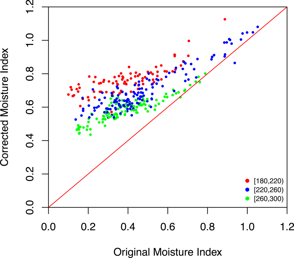
Figure 8. Scatter plot showing the impact of the [CO2] correction on the reconstructed moisture index (MI). The colored dots represent the implied change in the reconstructions, grouped according to level of the actual [CO2] at that time (in ppm).
The direct impact of low [CO2] on tree growth accounts for the relatively low abundance of mesophytic and Mediterranean trees during the glacial. Reconstructed MI is somewhat higher than today. Nevertheless, intervals of increasing MI during the glacial—as in the first part of MIS 2—are marked by a decrease in steppe taxa and an increase in conifers. The increase in Mediterranean taxa during the later Holocene, at a time when reconstructed MI indicates progressive drying, reflects the reconstructed strong insolation-driven winter warming through the Holocene because Mediterranean trees occur at areas with intermediate levels of water availability, but are sensitive to winter temperature (Harrison et al., Reference Harrison, Prentice, Sutra, Barboni, Kohfeld and Ni2010).
Several abrupt changes are shown in the reconstructions, particularly during MIS 5a and in the glacial period. Some of these (Supplementary Fig. 3) occur at times that correspond to D-O events, as identified from Greenland ice core records (Dansgaard et al., Reference Dansgaard, Johnsen, Clausen, Dahl-Jensen, Gundestrup, Hammer, Oeschger, Hansen and Takahashi1984; Steffensen et al., Reference Steffensen, Andersen, Bigler, Clausen, Dahl-Jensen, Fischer and Goto-Azuma2008), including D-O 20 (72.28–70.28 cal ka) and D-O 19 (76.4–74 cal ka) in MIS 5a, and D-O 9 (40.11–39.81 cal ka) and D-O 8 (38.17–36.57 cal ka) in MIS 3 (for dating see Wolff et al., Reference Wolff, Chappellaz, Blunier, Rasmussen and Svensson2010). Heinrich Stadial 2 (26.45–24.25 cal ka) (Sanchez Goñi and Harrison, Reference Sánchez Goñi and Harrison2010) also corresponds to an interval of year-round cooling in our reconstructions. Gaps in the pollen record, and poor dating resolution in some parts of the record, preclude identification of other D-O and Heinrich events. The limitations of the age model mean that even the correspondence between abrupt changes registered in El Cañizar de Villarquemado and the Greenland D-O events is uncertain. Nevertheless, where abrupt D-O like events are registered, they were characterized by increased seasonality, which may contribute to the high seasonality recorded during some periods during the glacial (Fig. 6).
DISCUSSION AND CONCLUSION
The El Cañizar de Villarquemado record is characterized by rapid warming in winter temperature of >5°C and an increase in growing-season warmth of >4000 degree days over a period of ca. 2–3 kyr during the transition from MIS 6 to MIS 5e. Although there are fluctuations, there is an overall decline in both summer and winter temperatures through MIS 5. However, there is a long interval with poor pollen preservation during MIS 5b, which limits our ability to gain a complete picture of the evolution of climate during this interval. Temperature reconstructions for MIS 4, 3, and 2 are not significantly lower than the end of MIS 5, but this might be because the coldest intervals occurred during the intervals of low pollen preservation in MIS 3 and 2. The Younger Dryas interval is marked by relatively cold summers (Supplementary Table 3). There was a gradual warming in both summer and winter through the Holocene. The broad-scale changes in moisture are coherent with changes in GDD0, with warmer summer intervals characterized by drier conditions and colder summers by wetter conditions. The MI reconstructions apparently indicate that the whole of the past ca. 130 kyr was wetter than today, although it is likely that the intervals of poor pollen preservation (for which we were unable to make reconstructions) were at least as arid as today. Rapid millennial-scale changes in temperature and moisture are superimposed on these longer-term trends, though not all D-O events can be identified in the record.
Many features of the El Cañizar de Villaquemado record are also shown in other quantitative reconstructions from the Mediterranean region. Both the Monticchio (Allen and Huntley, Reference Allen and Huntley2009) and the Lake Ohrid (Sinopoli et al., Reference Sinopoli, Peyron, Masi, Holtvoeth, Francke, Wagner and Sadori2019) records show rapid warming at the transition from MIS 6 to MIS 5e. This warming occurs over a longer period in the Monticchio (ca. 5 kyr) and Ohrid (ca. 7 kyr) records. The apparent rapidity of this transition at El Cañizar de Villarquemado could reflect age-model uncertainties and/or regional idiosyncrasies in the vegetation composition. Differences between the sub-stages of MIS 5 are more pronounced in the Monticchio and Ohrid records than at El Cañizar de Villarquemado. Comparison of the modern analogue and WA-PLS reconstructions at Lake Ohrid shows that modern-analogue reconstructions (and, by implication, the response-surface approach used at Monticchio) tend to produce stronger fluctuations, which might contribute to explaining the more muted variability at El Cañizar de Villarquemado. However, the pronounced cold, dry interval registered in Monticchio and Ohrid during MIS 5b corresponds to an interval of low pollen preservation in Villarquemado. This, and the fact that the El Cañizar de Villarquemado site lies at the warmer and drier end of the climate gradient across the Mediterranean, could contribute to the apparent differences between the sites.
The coldest interval at Monticchio during MIS 2 is also represented by an hiatus in Villarquemado. The Younger Dryas was characterized by cooler summers and wetter conditions at Villarquemado, but only a small decrease in winter temperature. The wetter conditions and the muted winter temperature response are consistent with the record from Monticchio (Allen and Huntley, Reference Allen and Huntley2009). However, the Holocene record from Monticchio is very different, showing summer cooling and relatively stable moisture levels after 10 ka. Thus, while there are some similarities between the available quantitative records from the Mediterranean, they each show distinctive features. These might reflect differences in the size and geomorphic setting of the three lakes, and hence the pollen source area (Sugita, Reference Sugita1984; Prentice, Reference Prentice1985; Prentice et al., Reference Prentice, Huntley and Webb1988) and, by implication, the geographic region represented by the climate reconstructions, but it is more likely that they reflect the pattern of climate changes across the region, as also indicated by qualitative information from other paleoclimate records (e.g., Harrison et al., Reference Harrison, Yu, Vassiljev, Wefer, Berger, Behre and Jansen2002; Roberts et al., Reference Roberts, Stevenson, Davis, Cheddadi, Brewster, Rosen, Battarbee, Gasse and Stickley2004, Reference Roberts, Jones, Benkaddour, Eastwood, Fillippi, Frogley and Lamb2008; Lechleitner et al., Reference Lechleitner, Amirnezhad-Mozhdehi, Columbu, Comas-Bru, Labuhn, Pérez-Mejías and Rehfeld2018).
The temperature record at El Cañizar de Villarquemado shows intervals of enhanced seasonality during MIS 5 and MIS 1, largely, but not entirely, driven by changes in GDD0. We have shown that there is a good correlation between these intervals of enhanced seasonality and orbitally forced changes in summer insolation during interglacial intervals. Temperature seasonality during the glacial was higher than during the interglacials and cannot be explained by insolation, although the within-glacial trends in seasonality do follow the changes in insolation. Izumi et al. (Reference Izumi, Bartlein and Harrison2013) showed that increased temperature seasonality at the last glacial maximum (LGM) compared to present, particularly in the northern extratropics, was a response to year-round forcing. They subsequently argued (Izumi et al., Reference Izumi, Bartlein and Harrison2014) that this was a consequence of changes in land-ocean and high-low latitude temperature gradients rather than an independent temperature response to the large-scale forcing. Rehfeld et al. (Reference Rehfeld, Münch, Ho and Laepple2018), using a network of terrestrial and marine records, showed a fourfold decrease globally in temperature seasonality from the LGM into the Holocene. While this global decrease is larger than indicated at El Cañizar de Villarquemado, Rehfeld et al. (Reference Rehfeld, Münch, Ho and Laepple2018) pointed out that the change is larger at higher northern latitudes and negligible in the tropics. Thus, the higher seasonality during the glacial than during interglacials reconstructed at El Cañizar de Villarquemado appears to be a robust feature. Enhanced seasonality at El Cañizar de Villarquemado is also associated with intervals of abrupt warming that correlate with D-O events (e.g., D-O 9). However, enhanced seasonality during the D-O events appears to have been driven primarily by changes in winter temperature. Changes in MI on both orbital and millennial timescales are generally anti-correlated with changes in GDD0 presumably because increased summer temperature and/or increased length of the growing season led to increased evapotranspiration and hence reduced MI.
There are gaps in the palynological record from El Cañizar de Villarquemado because of intervals of poor pollen preservation during MIS 5b, MIS 3, and MIS 2 (Fig. 3). The sedimentological record suggests that these were arid intervals, characterized by alluvial fan rather than lacustrine deposition, and oxidation of the sediments. A speleothem record from El Pindal (Moreno et al., Reference Moreno, Stoll, Jiménez Sánchez, Cacho, Valero-Garcés, Ito and Edwards2010) also shows hiatuses in formation during MIS 2, consistent with our interpretation that the depositional hiatus at El Cañizar de Villarquemado is indicative of aridity. Similar situations have been identified in other palynological sequences from the region during arid intervals (Valero-Garcés et al., Reference Valero-Garcés, González-Sampériz, Delgado-Huertas, Navas, Machín and Kelts2000, Reference Valero-Garcés, González-Sampériz, Navas, Machín, Delgado-Huertas, Peña-Monne, Sancho-Marcén, Stevenson and Davis2004; González-Sampériz et al., Reference González-Sampériz, Valero-Garcés and Carrión2004, Reference González-Sampériz, Valero-Garcés, Carrión, Peña-Monné, García-Ruiz and Martí-Bono2005; Vegas-Villarubía et al., Reference Vegas-Vilarrúbia, González-Sampériz, Morellón, Gil-Romera, Pérez-Sanz and Valero-Garcés2013). Hyper-arid periods are a problem for pollen preservation and, while further work may improve the pollen record at El Cañizar de Villarquemado, it is unlikely that we will be able to obtain a quantitative record of climate during such intervals. Nevertheless, El Cañizar de Villarquemado provides a relatively complete and well-dated record from continental Iberia (González-Sampériz et al., Reference González-Sampériz, Leroy, Carrión, Fernández, García-Antón, Gil-García, Uzquiano, Valero-Garcés and Figueiral2010, Reference González-Sampériz, Gil-Romera, García-Prieto, Aranbarri, Moreno, Morellón and Sevilla-Callejo2020; Moreno et al., Reference Moreno, González-Sampériz, Morellón, Valero-Garcés and Fletcher2012; Valero-Garcés et al., Reference Valero-Garcés, González-Sampériz, Gil-Romera, Benito, Moreno, Oliva-Urcia and Aranbarri2019) and it is important to document changes in the drier part of the circum-Mediterranean region.
All reconstruction methods that use modern pollen-climate relationships are sensitive to the choice of training datasets, vegetation diversity, and the potential absence of analogue assemblages (Gavin et al., Reference Gavin, Oswald, Wahl and Williams2003; Jackson and Williams, Reference Jackson and Williams2004; Bartlein et al., Reference Bartlein, Harrison, Brewer, Connor, Davis, Gajewski and Guiot2011). While the training dataset that we have used provides a good coverage of Europe, Morocco, and the Middle East, it lacks modern pollen from much of northern Africa. However, it contains more than 6000 samples and includes samples from very cold and very warm environments to allow reconstruction of climate both much warmer and much colder than today (Turner et al., Reference Turner, Wei, Prentice and Harrison2020). Analysis of the GAMs for individual taxa also shows that they have ecologically plausible relationships with climate variables (Wei et al., Reference Wei, Prentice and Harrison2020). Furthermore, uncertainty estimates on the reconstructions, calculated using a method that propagates the calibration errors from the modern training dataset into the down-core reconstructions by assessing the calibration error associated with the particular assemblage in an individual pollen sample, are generally rather small. We have shown that pollen preservation issues, as indicated by intervals when the number of indeterminable grains was higher than average, do not affect our reconstructions. However, our analyses show that intervals of very low biodiversity are often characterized by more extreme values than other intervals. We have taken this into account by screening the down-core samples and excluding samples with very low diversity.
Much of the discussion about the lack of modern analogues has focused on interpretation of assemblages of species that are not found together today (Overpeck et al., Reference Overpeck, Webb and Prentice1985; Jackson and Williams, Reference Jackson and Williams2004; Williams and Shuman, Reference Williams and Shuman2008). However, one important non-analogue situation that is ignored in all previous statistical reconstructions is the impact of [CO2] different from today on plant assemblages, with important effects on apparent climatic moisture inferred from pollen data (Prentice et al., Reference Prentice, Cleator, Huang, Harrison and Roulstone2017; Cleator et al., Reference Cleator, Harrison, Nichols, Prentice and Roustone2019). Taking the impact of [CO2] into account in our reconstructions reduces the variability of MI during glacial intervals. Prentice et al. (Reference Prentice, Cleator, Huang, Harrison and Roulstone2017) showed that this correction produced a reconciliation of apparently contradictory interpretations of pollen and geomorphic data for hydroclimatic changes in southeastern Australia at the LGM. High lake levels coincident with steppic vegetation are a feature of several glacial records from the Mediterranean region, including the Padul record (Camuera et al., Reference Camuera, Jiménez-Moreno, Ramos-Román, García-Alix, Toney, Anderson and Jiménez-Espejo2018, Reference Camuera, Jiménez-Moreno, Ramos-Román, García-Alix, Toney, Anderson and Jiménez-Espejo2019) and sequences from northeastern Iberia, such as the playa lakes of the Central Ebro Basin (Valero-Garcés et al., Reference Valero-Garcés, González-Sampériz, Delgado-Huertas, Navas, Machín and Kelts2000, Reference Valero-Garcés, González-Sampériz, Navas, Machín, Delgado-Huertas, Peña-Monne, Sancho-Marcén, Stevenson and Davis2004; González-Sampériz et al., Reference González-Sampériz, Valero-Garcés and Carrión2004, Reference González-Sampériz, Valero-Garcés, Carrión, Peña-Monné, García-Ruiz and Martí-Bono2005). Camuera et al. (Reference Camuera, Jiménez-Moreno, Ramos-Román, García-Alix, Toney, Anderson and Jiménez-Espejo2019) argued that this reflects low evapotranspiration because of the low temperatures. However, much larger changes in temperature than implied by the El Cañizar de Villarquemado record would be required (e.g., Prentice et al., Reference Prentice, Guiot and Harrison1992). A simpler explanation is that the abundance of xerophytes and the reduction in trees reflect the ecophysiology impact of low [CO2].
The El Cañizar de Villarquemado reconstructions provide a detailed picture of the response of western Mediterranean climate and vegetation to changes in external forcing in this sensitive region over a long period of time. It would be useful to generate quantitative reconstructions from other long records because preliminary comparisons with Lago di Monticchio and Lake Ohrid indicate some complexity in the response of climate to changes in external forcing within the circum-Mediterranean region. However, given that the largest impact of glacial-interglacial changes in atmospheric circulation is likely to be on precipitation and plant-available moisture, it will be important to take account of the impact of changing [CO2] in these reconstructions.
ACKNOWLEDGMENTS
DW and SPH acknowledge support from the ERC-funded project GC2.0 (Global Change 2.0: Unlocking the past for a clearer future, grant no. 694481). PG-S, GG-R, and SPH acknowledge support from the Spanish Ministerio de Economia y Competitividad for the project CGL2015-69160R “Dinámica, Monitorización y Calibración de la vegetación Mediterránea en respuesta al Calentamiento Global en series temporales largas (DINAMO3),” as well as for CGL2012-33063 and CGL2009-07992. ICP acknowledges support from the ERC-funded project “Re-inventing Ecosystem and Land-surface Models (REALM),” grant no. 787203. This research is a contribution to the Imperial College initiative on Grand Challenges in Ecosystems and the Environment (ICP). We thank Jon Lloyd for advice on the implementation of convex hulls, and Maria Dance for the implementation of GWR. We also thank the PaleoIPE team for multi-proxy reconstruction and discussion regarding the El Cañizar de Villarquemado sequence; Maria Leunda, Josu Aranbarri, and Héctor Romanos for providing additional surface pollen samples; and Miguel Sevilla Callejo for the Iberian Peninsula and El Cañizar de Villarquemado vegetation maps of Figure 2. We thank Patrick Bartlein and Hugues-Alexandre Blain for helpful comments on the manuscript.
SUPPLEMENTARY MATERIAL
The supplementary material for this article can be found at https://doi.org/10.1017/qua.2020.108


 Open access