


1. Introduction
Since the original work of Taylor (Reference Taylor1953), the notion of an effective diffusion has proven to be extremely useful. His theory, and extensions thereof (Aris & Taylor Reference Aris and Taylor1956; Brenner Reference Brenner1980; Brenner & Adler Reference Brenner and Adler1982), has become the standard for estimating the dispersion in systems ranging from transport in blood (Goldstick, Ciuryla & Zuckerman Reference Goldstick, Ciuryla and Zuckerman1976; Scow, Blanchette-Mackie & Smith Reference Scow, Blanchette-Mackie and Smith1976; Eckstein & Belgacem Reference Eckstein and Belgacem1991) and groundwater systems (Desaulniers et al. Reference Desaulniers, Kaufmann, Cherry and Bentley1986; Zheng & Wang Reference Zheng and Wang1999), sugar transport in plants (Jensen et al. Reference Jensen, Rio, Hansen, Clanet and Bohr2009, Reference Jensen, Berg-Sørensen, Bruus, Holbrook, Liesche, Schulz, Zwieniecki and Bohr2016; Dölger et al. Reference Dölger, Rademaker, Liesche, Schulz and Bohr2014), and the dispersion of airborne droplets for spreading in disease transmission (Eames et al. Reference Eames, Tang, Li and Wilson2009; Hui et al. Reference Hui, Chow, Chu, Ng, Hall, Gin and Chan2009; Liu et al. Reference Liu, Wei, Li and Ooi2017). Therefore, dispersion has been the focus of much experimental, numerical and theoretical research. The understanding of dispersion in axially invariant channels has since Taylor (Reference Taylor1953) and Aris & Taylor (Reference Aris and Taylor1956) been extended to allow for alternating fluid boundary conditions (Adrover & Cerbelli Reference Adrover and Cerbelli2017; Adrover, Cerbelli & Giona Reference Adrover, Cerbelli and Giona2018) and boundaries absorbing the solute (Levesque et al. Reference Levesque, Bénichou, Voituriez and Rotenberg2012; Dagdug, Berezhkovskii & Skvortsov Reference Dagdug, Berezhkovskii and Skvortsov2014). However, most channels and pores in natural and industrial systems are not perfectly flat. The addition of a varying boundary geometry is found to result in significant increase for the dispersion (Rosencrans Reference Rosencrans1997; Drazer et al. Reference Drazer, Auradou, Koplik and Hulin2004; Schmidt, McCready & Ostafin Reference Schmidt, McCready and Ostafin2005; Bolster, Dentz & Le Borgne Reference Bolster, Dentz and Le Borgne2009; Bouquain et al. Reference Bouquain, Méheust, Bolster and Davy2012), and for certain systems even results in a decrease of the asymptotic spreading (Rosencrans Reference Rosencrans1997; Drazer et al. Reference Drazer, Auradou, Koplik and Hulin2004; Bolster et al. Reference Bolster, Dentz and Le Borgne2009). Brenner's theory (Brenner Reference Brenner1980; Brenner & Adler Reference Brenner and Adler1982) has proven to be a solid theoretical framework for investigating such geometries (Bolster et al. Reference Bolster, Dentz and Le Borgne2009).
Most of the previous work with varying aperture has been done under certain idealized conditions, such as with potential flow (Eames & Bush Reference Eames and Bush1999; Choi et al. Reference Choi, Margetis, Squires and Bazant2005) or in the low-Reynolds-number regime where inertial effects can be ignored. Bolster et al. (Reference Bolster, Dentz and Le Borgne2009) studied solute dispersion in channels with sinusoidal wall roughness under Stokes flow conditions. Here, the linearity of Stokes’ equations and the analyticity of the boundary allowed for a perturbative approximation to the dispersion coefficient. Bouquain et al. (Reference Bouquain, Méheust, Bolster and Davy2012) built upon this work by investigating the effects of fluid inertia on the effective solute transport. Inertial effects can result in low-velocity regions called recirculation zones (RZ), which can trap the solute (Buonocore, Sen & Semperlotti Reference Buonocore, Sen and Semperlotti2020), resulting in a significant increase in the asymptotic spreading. While RZ can occur in Stokes flow, they become more dominant with increasing Reynolds number and appear for much smaller geometrical constraints.
Although the smooth single-wavelength roughness considered in a number of works (Laachi et al. Reference Laachi, Kenward, Yariv and Dorfman2007; Yariv & Dorfman Reference Yariv and Dorfman2007; Bolster et al. Reference Bolster, Dentz and Le Borgne2009; Bouquain et al. Reference Bouquain, Méheust, Bolster and Davy2012) represents a major step towards real-world applications, the wall profiles found in both natural rock fractures (Cvetkovic, Selroos & Cheng Reference Cvetkovic, Selroos and Cheng1999; Fiori & Becker Reference Fiori and Becker2015) and microfluidic devices such as the staggered herringbone mixer (Williams, Longmuir & Paul Reference Williams, Longmuir and Paul2008; Ottino et al. Reference Ottino, Wiggins, Stroock and McGraw2004) do not obey the same smoothness, but contain jumps and often rugged shapes. Rough surfaces have been studied for purely diffusive transport (Mangeat, Guérin & Dean Reference Mangeat, Guérin and Dean2018), including geometries similar to those studied here (Kalinay & Percus Reference Kalinay and Percus2010; Dagdug et al. Reference Dagdug, Berezhkovskii, Zitserman and Bezrukov2021). With the addition of flow, recently Yoon & Kang (Reference Yoon and Kang2021) applied advected random walk simulations to investigate the combined effect of a self-similar roughness and fluid inertia for a variety of advective transport rates. However, it was limited to the transient regime. Dagdug et al. (Reference Dagdug, Berezhkovskii and Skvortsov2014) studied how dispersion is affected by narrow dead ends where particles may be trapped for a finite time. Larger openings may lead to non-negligible flow inside the dead ends and non-trivial flow profiles. Further, the role of dead ends for diffusion with constant drift has been studied (Laachi et al. Reference Laachi, Kenward, Yariv and Dorfman2007; Berezhkovskii et al. Reference Berezhkovskii, Dagdug, Makhnovskii and Zitserman2010; Berezhkovskii & Dagdug Reference Berezhkovskii and Dagdug2011; Zitserman et al. Reference Zitserman, Berezhkovskii, Antipov and Makhnovskii2014). However, this does not account for the role of fluid shear or Reynolds number. Despite the ubiquity of rough surfaces and high-inertia flows, it is unclear exactly how together they influence the effective diffusion. This is particularly important as numerous previous studies assume negligible flow in the stagnant areas or ignore fluid shear. The main novelty of this study is that we consider a geometry with sharply changing boundary roughness, resulting in large RZ. Previous studies of dispersion in channels of varying apertures have been limited to smooth boundaries (Bolster et al. Reference Bolster, Dentz and Le Borgne2009; Bouquain et al. Reference Bouquain, Méheust, Bolster and Davy2012) or ignore both large openings and the flow inside the stagnant areas (Laachi et al. Reference Laachi, Kenward, Yariv and Dorfman2007; Berezhkovskii et al. Reference Berezhkovskii, Dagdug, Makhnovskii and Zitserman2010; Berezhkovskii & Dagdug Reference Berezhkovskii and Dagdug2011; Levesque et al. Reference Levesque, Bénichou, Voituriez and Rotenberg2012; Dagdug et al. Reference Dagdug, Berezhkovskii and Skvortsov2014; Zitserman et al. Reference Zitserman, Berezhkovskii, Antipov and Makhnovskii2014). In this paper, we show that this boundary roughness leads to a qualitatively different behaviour compared to the aforementioned studies.
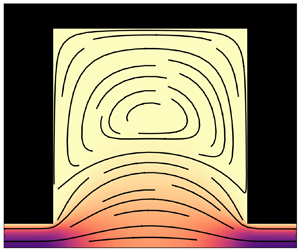
In order to understand this, we investigate systematically how a periodic discontinuous rough square boundary, illustrated in figure 1, influences the flow and effective diffusion of a passive solute in a two-dimensional channel. The channel is defined solely by the dimensionless boundary roughness amplitude  $b$ with average channel half-width
  $a$. The geometry is a simplified representation of generic rough-walled channels containing sharp notches and grooves of various sizes, e.g. discontinuous jumps in the boundary profile. The goal is to find and explain the effective diffusion coefficient's dependency on the boundary amplitude, Péclet and Reynolds number. The main result of the paper is a previously unobserved decrease in the effective diffusion coefficient with increasing Reynolds number, which is explained through the RZ trapping more solute particles into effectively stationary regions at larger Reynolds numbers, reducing the correlation time of horizontal solute transport.

Figure 1. Illustration of the geometry considered in this paper. The quadratic square rough channel consists of infinitely many repeated unit cells, with channel height  $2a+r$, unit cell width
  $2r$, and unit cell area
  $4a^2b$. The fluid unit cell boundary is created from the union of the unit cell boundary and wall boundary (2.8). The dimensionless square roughness
  $b\equiv r/a$ characterizes the geometry fully. For
  $b=0$, one finds Aris’ channel, and for
  $b=2$, the channel is completely closed.
The paper is organized as follows. In § 2, we summarize the necessary theory, and in § 3, we describe the geometry and numerical procedure underlying our computations. The results on flow fields and effective diffusion coefficients are presented in § 4, and in § 5 we summarize and conclude.
2. Theory
Passive transport of diffusive particles can be described by the evolution of the concentration field  $C(\boldsymbol {r}, t)$ in space
  $\boldsymbol {r}$ and time
  $t$, which is governed by the advection–diffusion equation,
 \begin{equation} \partial_t C = \mbox{Pe}^{-1}\,\nabla^2 C - \boldsymbol{u} \boldsymbol{\cdot} \boldsymbol{\nabla} C. \end{equation}
The equation is written in dimensionless form, with incompressible flow and a constant molecular diffusion coefficient  $D_m$. The Péclet number
  $\mbox{Pe}$ is a dimensionless number that measures the advective versus diffusive transport rate
  $\mbox{Pe}\equiv aU/D_m$, where
  $U$ is the average streamwise velocity and
  $a$ is the mean channel half-width. The velocity field
  $\boldsymbol {u}$ is determined by solving the steady incompressible Navier–Stokes equations
 \begin{equation} \boldsymbol{u}\boldsymbol{\cdot}\boldsymbol{\nabla}\boldsymbol{u} ={-}\boldsymbol{\nabla}P + \mbox{Re}^{-1}\,\nabla^2\boldsymbol{u} + \boldsymbol{f},\quad \boldsymbol{\nabla}\boldsymbol{\cdot}\boldsymbol{u}=0. \end{equation}
Here,  $P$ is the pressure, and
  $\boldsymbol {f}$ is an external horizontal body force. The equation is written in dimensionless form, with the Reynolds number
  $\mbox{Re}$ relating the inertial and viscous forces defined as
  $\mbox{Re}\equiv Ua/\nu$, where
  $\nu$ is the kinematic viscosity. To achieve a stationary velocity field, necessary for the application of Brenner's theory, the time-derivative term in the Navier–Stokes equations is ignored. For the simulations at
  $\mbox{Re}=0$, we also neglect the nonlinear term
  $\boldsymbol {u}\boldsymbol {\cdot }\boldsymbol {\nabla }\boldsymbol {u}$.
By solving (2.1) without flow and geometric constraints, one finds that the positional variance of the concentration  $\sigma ^2$ in a given direction grows linearly in time with slope
  $2D_m$. The effective diffusion coefficient parallel to the flow in
  $d$ dimensions, with
  $x$ being the streamwise spatial coordinate, can therefore be defined as
 \begin{equation} \sigma^2_\parallel(t) \equiv \int_{\mathbb{R}^d} x^2\,P(\boldsymbol{r}) \,\mathrm{d}^d \boldsymbol{r} - \left(\int_{\mathbb{R}^d} x \,P(\boldsymbol{r}) \,\mathrm{d}^d \boldsymbol{r}\right)^2 \equiv 2D_{{\parallel}}t, \end{equation}
where the probability  $P$ is the normalized concentration. The linear scaling is expected to hold when the solute has traversed the channel height multiple times, i.e. when
  $a^2/D_m \ll t$. The effective diffusion coefficient
  $D_\parallel$ will depend on the flow and geometry.
Brenner (Reference Brenner1980) devised a general theoretical framework for calculating the effective diffusion coefficient in an arbitrary periodic geometry with steady incompressible flow. In this theory, the effective diffusion coefficient for dispersion along  $x$ can be found by calculating
 \begin{equation} D_{{\parallel}} = D_m \left\langle 1 - 2\,\frac{{\partial}\chi}{{\partial}x} + |\boldsymbol{\nabla} \chi|^2 \right\rangle, \end{equation}
where the angle brackets denote a spatial average, defined in two dimensions as
 \begin{equation} \langle f \rangle = \frac{1}{V_\varOmega} \int_\varOmega f(\boldsymbol{r})\,\mathrm{d} \boldsymbol{r}^2, \end{equation}
with  $V_\varOmega$ being the volume of the unit cell. The scalar field
  $\chi$ is the solution of the equation
 \begin{equation} \nabla^2 \chi - \mbox{Pe}\,\boldsymbol{u} \boldsymbol{\cdot} \boldsymbol{\nabla} \chi = \mbox{Pe}\,\hat{\boldsymbol{x}} \boldsymbol{\cdot}\boldsymbol{u}', \end{equation}
where  $\hat {\boldsymbol {x}}$ is the unit vector in the streamwise direction, and
  $\boldsymbol {u}'$ is the velocity profile in the reference frame following the mean velocity,
  $\boldsymbol {u}' = \boldsymbol {u}-\langle \boldsymbol {u}\rangle$. The scalar field must also satisfy the boundary condition
 \begin{equation} \hat{\boldsymbol{n}} \boldsymbol{\cdot} \boldsymbol{\nabla} \chi ={-} \hat{\boldsymbol{n}} \boldsymbol{\cdot} \hat{\boldsymbol{x}} \quad\text{on}\ \partial\varOmega_{{wall}}. \end{equation}
The solution must also be periodic on  $\partial \varOmega _{{cell}}$, which together with
  $\partial \varOmega _{{wall}}$ constitutes the boundary of the unit cell:
 \begin{equation} \partial\varOmega = \partial \varOmega_{{cell}}\cup \partial \varOmega_{{wall}}. \end{equation}
This is illustrated in figure 1. Additionally, we may remove the gauge freedom in  $\chi$ by requiring
  $\left \langle \chi \right \rangle = 0.$
Brenner's result is a generalization of Aris’ solution (Aris & Taylor Reference Aris and Taylor1956), which is valid only for axially invariant channels. Axially invariant geometry results in a horizontal velocity field  $\boldsymbol {u} = u_x \hat {\boldsymbol { x}}$, and
  $\chi$ becoming independent of
  $x$, i.e.
  $\chi (\boldsymbol {r}) = \chi (\boldsymbol {r}_\perp )$, where the subscript
  $\perp$ denotes the coordinates orthogonal to the flow direction. From these simplifications, we find a special case of Brenner's equation (2.4),
 \begin{equation} D_{{\parallel}}^{Aris} = D_m \left( 1 + \left\langle |\boldsymbol{\nabla}_\perp \chi(\boldsymbol{r}_\perp)|^2 \right\rangle \right), \end{equation}
where the scalar field is the solution of the simpler equation
 \begin{equation} \nabla^2_\perp \chi =\mbox{Pe}\,\hat{\boldsymbol{x}} \boldsymbol{\cdot}\boldsymbol{u}'. \end{equation}
By introducing the dimensionless quantity  $\phi$ through
  $\chi = a\,\mbox{Pe}\,\phi$, (2.9) becomes
 \begin{equation} D_{{\parallel}}^{Aris} = D_m \left[1 + \mbox{Pe}^2 \left\langle |\boldsymbol{\nabla} \phi|^2 \right\rangle \right]. \end{equation}
By defining a geometric factor  $\kappa =\left \langle |\boldsymbol {\nabla } \phi |^2 \right \rangle$, the result can be written identically to Aris’ expression (Aris & Taylor Reference Aris and Taylor1956, p. 75), with
  $\kappa = 2/105$ for a straight two-dimensional channel.
To simulate the trajectories of the diffusive passive tracers and verify independently the theoretical predictions made with Brenner's theory, advected random walk simulations are used (Bolster et al. Reference Bolster, Dentz and Le Borgne2009, Reference Bolster, Méheust, Le Borgne, Bouquain and Davy2014; Giona, Venditti & Adrover Reference Giona, Venditti and Adrover2020). The discretization method, boundary conditions and numerical implementation are discussed in Appendix A.
3. Velocity fields, geometry and problem setup
Following the result from Aris (Aris & Taylor Reference Aris and Taylor1956), among others (Bolster et al. Reference Bolster, Dentz and Le Borgne2009; Bouquain et al. Reference Bouquain, Méheust, Bolster and Davy2012), we represent the effective diffusion coefficient in the form
 \begin{equation} D_{{\parallel}} = D_m\left(\frac{d_m^{{\parallel}}(b)}{D_m}+\kappa\,\mbox{Pe}^2\,g\left(\mbox{Pe}, \mbox{Re}, b \right)\right). \end{equation}
The geometric factor  $g$ measures the effect of fluid flow on the asymptotic spreading as a function of the Péclet number, Reynolds number and roughness amplitude
  $b$. The constant
  $\kappa$ is the geometric factor from the Taylor–Aris result, which for a two-dimensional straight channel takes the value
  $2/105$, such that
  $g(\mbox{Pe}, \mbox{Re}, 0 )=1$. We have further defined
  $d_m^{\parallel }(b)$ as the effective diffusion coefficient for pure diffusion at roughness
  $b$, such that one retrieves the correct value in the limit of zero
  $\mbox{Pe}$. The effective diffusion has therefore been decomposed into one term,
  $d_m^{\parallel }(b)$, representing the effect of horizontal purely diffusive transport that is important at small Péclet numbers, and another term representing the effect of flow, where a scaling of order
  $\mbox{Pe}^2$, similar to Taylor–Aris, is expected.
To understand dispersion phenomena in rough channels, the velocity field is found by solving numerically the incompressible time-independent Navier–Stokes equations for various boundary amplitudes and Reynolds numbers. After solving for the velocity profile, the Reynolds number is calculated and the flow is normalized to have horizontal unit cell average velocity  $1$. The Reynolds number is therefore changed by varying the kinematic viscosity
  $\nu$. Different transport rates are investigated in a wide range of Péclet numbers, where the diffusion coefficient is varied upon the same velocity profile. By altering the diffusivity of momentum and mass, the Reynolds and Péclet numbers are changed independently. Hence the investigation is performed for various Schmidt numbers, defined as
  $\mbox{Sc}\equiv \mbox{Pe}/\mbox{Re}$. Experimentally, the Péclet number can remain fixed while increasing the Reynolds number by reducing the viscosity of the fluid, and increasing the average velocity to compensate for a larger molecular diffusivity. This can be seen from the Stokes–Einstein relation (Einstein Reference Einstein1905) where
  $D_m\propto 1/\nu$.
The study is purely numerical, primarily using the finite element method. Convergence is verified by ensuring that the average velocity and effective diffusion coefficient change by less than  $1\,\%$ when doubling the spatial resolution of the finite element mesh. The code for the Navier–Stokes equations, Brenner's equation and diffusive passive tracers simulations are public through a designated GitHub repository (Haugerud Reference Haugerud2022). The variational form of the equations is discussed in Appendix B.
4. Results
4.1. Velocity field
In figure 2, the streamlines in the bottom half of the unit cell are visualized for roughnesses  $b=0.4$,
  $0.8$ and
  $1.6$, for Reynolds numbers
  $0$ (figure 2a–c) and
  $10^{1.5}\approx 32$ (figure 2d–f). For
  $b=0.4$, the RZ are close to filling the full cavity area, independent of Reynolds number. With increasing roughness, the high-speed central streamlines move further into the cavities at low
  $\mbox{Re}$, reducing the relative size of the RZ. This does not occur for
  $\mbox{Re}=32$, where the RZ fill the entire cavity area for all boundary amplitudes.

Figure 2. Visualization of the velocity fields at different roughnesses  $b$ and Reynolds numbers. For each panel, the spatial axes are scaled equally, and the colour bar denotes the fluid speed in factors of the unit cell average value. (a–c) Reynolds number
  $0$, and roughness
  $b=0.4$,
  $0.8$ and
  $1.6$, respectively. (d–f) Reynolds number
  $32$, and roughness
  $b=0.4$,
  $0.8$ and
  $1.6$, respectively.
4.2. Verification: comparisons between Brenner's solution and diffusive passive tracers
The numerical implementation of the solver for Brenner's equations (2.6) and (2.7) is verified by comparing its predicted effective diffusion coefficient with those found using advected random walk simulations, as shown in figure 3. The comparison without flow, shown in figure 3(a), shows that the effective diffusion coefficient decreases linearly until around  $b=1$ with slope
  $-0.42$, and approaches zero when the channel is completely closed at
  $b=2$. The result is compared further to the theories due to Fick–Jacobs (Jacobs Reference Jacobs1935) and Dagdug et al. (Reference Dagdug, Berezhkovskii, Zitserman and Bezrukov2021). While Fick–Jacobs overestimates and Dagdug et al. underestimates the effective diffusion coefficient, the latter is much closer to the correct values produced by Brenner's theory. This is understood by the former being valid only for slowly varying boundaries, and the latter being valid even for abruptly varying channel diameters (Dorfman & Yariv Reference Dorfman and Yariv2014). All methods agree when the narrowest channel width approaches zero, as the horizontal transport is then dominated by this portion of the channel. For the case with flow, shown in figure 3(b), the roughness results in a large increase for small values of the Péclet number, which approaches a scaling with the Péclet number similar to the Taylor–Aris expression (2.11). For
  $b=0$, the results also agree with the Taylor–Aris result. Based on this, we have established that the Brenner equations solver produces the correct effective diffusion coefficient. For the following results, the Brenner equations solver is used, as it is exact and computationally much more efficient than advected random walk simulations.

Figure 3. The effective diffusion coefficient (a) without advection and (b) with advection, at zero Reynolds number, found by different methods, i.e. solving Brenner's equation, random walk (RW) simulations and the analytic expressions from Fick–Jacobs (Jacobs Reference Jacobs1935) and Dagdug et al. (Reference Dagdug, Berezhkovskii, Zitserman and Bezrukov2021).
4.3. Effective diffusion for creeping flow
With a verified solver of Brenner's equations, the effective diffusion coefficient is calculated as a function of both the Péclet number and the roughness at creeping flow. The form of the geometric factor  $g$, defined in (3.1), at Stokes flow conditions (
 $\mbox{Re}=0$) is displayed as functions of Péclet number and roughness in figure 4. The figure shows that increasing the roughness always results in more efficient spreading, but the effect is diminished at higher Péclet numbers. Furthermore, the geometric factor is always larger than 1, meaning that an increase in the amplitude
  $b$ always increases the dispersion due to flow. For very large Péclet numbers,
  $g$ moves closer to
  $1$, i.e. more similar to the Taylor–Aris result.

Figure 4. At Reynolds number 0, the geometric factor (3.1) as functions of (a) Péclet number and (b) boundary roughness.
Even though the geometric factor is always larger than  $1$, the effective diffusion is not necessarily larger than the Taylor–Aris result from (2.11). In figure 5, the relative change in the dispersion from Poiseuille flow to our geometry, defined as
 \begin{equation} \Delta D_\parallel \equiv \frac{D_\parallel(\mbox{Pe}, b, \mbox{Re}=0)-D_\parallel^{aris}(\mbox{Pe})}{D_\parallel^{aris}(\mbox{Pe})}, \end{equation}
is displayed. A slight decrease is observed when both transport mechanisms are of equal importance,  $\mbox{Pe}=1$, due to the horizontal diffusive spreading being limited by the varying boundary amplitude. This is true only for small boundary amplitudes, and the relative change becomes positive at around
  $b=1.25$. The relative change is maximized for an intermediate value
  $\mbox{Pe} = 32$. Except for
  $\mbox{Pe}=10^3$, the relative change is largest for the largest boundary amplitude.

Figure 5. At Reynolds number 0, the relative change in the effective diffusion coefficient (4.1), compared to the Taylor–Aris result, is positive except at  $\mbox{Pe}=1$.
4.4. Effective diffusion with fluid inertia
The effect of fluid inertia on  $D_\parallel$ is displayed in figure 6, through its relative change from creeping flow to a non-zero Reynolds number:
 \begin{equation} \Delta D_\parallel^{{Re}} \equiv \frac{D_\parallel(\mbox{Pe}, b, \mbox{Re})-D_\parallel(\mbox{Pe},b,\mbox{Re}=0)}{D_\parallel(\mbox{Pe},b,\mbox{Re}=0)}. \end{equation}
For each panel of figure 6, the Péclet number is constant, while changing the flow through the roughness and Reynolds number. For small roughnesses the relative change is zero, independent of the Reynolds and Péclet numbers. When the two transport mechanisms are of equal importance, an increase in the Reynolds number increases the spreading, and this is further magnified with increasing roughness. On the contrary, for high Péclet numbers, the same change in flow decreases the value of the effective diffusion coefficient by as much as  $50\,\%$. The consequence of fluid inertia is therefore highly dependent on the relative transport rates.

Figure 6. The relative change in the effective diffusion coefficient with Reynolds number (4.2) is displayed for a constant Péclet number, while changing the flow through the roughness and Reynolds number.
4.5. Residence times of diffusive passive tracers
By analysing the positions and trajectories of the diffusive passive tracers, a physical explanation for the behaviour observed above can be found. We are especially interested in understanding how an increase in Reynolds number can increase or decrease the effective diffusion, depending on the Péclet number. Therefore, the simulations are performed at creeping flow and  $\mbox{Re}=32$ – the same values for which the streamlines in figure 2 are displayed. Three different orders of magnitudes of the Péclet number are also investigated,
  $1$,
$1$,  $10$ and
  $100$, corresponding to three of the graphs in figure 6.
By finding the shape of the RZ, the average number of particles in the RZ is measured and displayed in figure 7. The proportion of particles always increases for creeping flow, although the slope decreases for the largest boundaries. For Reynolds number  $32$, on the other hand, the linear increase matches the fact that the RZ fill the whole cavity area. This behaviour is consistent with the behaviour of the RZ area, inferred from figure 2. For both cases, the effect of changing the Péclet number is negligible compared to the fluctuations around the averaged values, as one would expect.

Figure 7. The average number of particles in RZ for  $\mbox{Re}=0$ (crosses) and
  $\mbox{Re}=32$ (dots) is displayed versus boundary roughness for a variety of Péclet numbers.
The probability density of residence times in the RZ and the central channel (CC) decays exponentially as  $P(t)=\exp (-t/\tau _i)$ for
  $i \in \{ CC, RZ\}$. For the set of Péclet numbers, Reynolds numbers and roughnesses investigated above, the behaviour of the characteristic residence times
  $\tau _{CC}$,
  $\tau _{RZ}$ are displayed in figure 8. With increasing Péclet number, the residence times in both the CC and the RZ increase due to the diffusive transport between the two regions diminishing. With a larger roughness, the RZ area increases and the CC area decreases, resulting in the same behaviour with their corresponding residence times. Increasing fluid inertia has a minimal effect on the RZ residence time, but drastically decreases the CC residence time, especially at large boundary amplitudes.

Figure 8. The characteristic residence times in (a) the recirculation zones  $\tau _{RZ}$, and (b) the central channel
  $\tau _{CC}$, for both creeping flow (dots) and inertial flow with
  $\mbox{Re}=32$ (crosses), with boundary roughness for a variety of Péclet numbers.
5. Discussion
To achieve a large value of the effective diffusion, the average autocorrelation time for the advected horizontal velocity should be maximized, with a broad distribution in advection speed between particles (Bolster et al. Reference Bolster, Dentz and Le Borgne2009). This can also be realized from the Taylor–Green–Kubo relation (Taylor Reference Taylor1922; Green Reference Green1951; Kubo Reference Kubo1957), which is an alternative way of retrieving the dispersion coefficient  $D_\parallel = \int _0^\infty C_v(t) \,\mathrm {d} t$, where
  $C_v = \overline {u'_x(t), u'_x(0)}$ is the ensemble averaged autocorrelation function for the streamwise Lagrangian velocity of the particles. A varying boundary geometry can result in a decrease in the effective diffusion coefficient due to the autocorrelation time being reduced with enhanced vertical diffusive transport at the pore throats. It can equally well increase due to the width of the velocity distribution increasing with additional fluid shear and RZ. This has been studied for smoothly varying boundary amplitudes (Bolster et al. Reference Bolster, Dentz and Le Borgne2009; Bouquain et al. Reference Bouquain, Méheust, Bolster and Davy2012), where a threshold value of the boundary amplitude is necessary for RZ to appear. RZ are present at all boundary amplitudes for the discontinuous geometry studied here, resulting in an effective diffusion coefficient larger than the Taylor–Aris result even at small boundary amplitudes, as shown in figure 5.
We observe that the geometric factor comes closer to the Taylor–Aris result for higher Péclet numbers, as seen in figure 4. The effect occurs at all roughnesses, but is enhanced at larger values. This result can seem surprising, as the Péclet number increases the importance of the flow field, which is highly dependent on the geometry. The behaviour can be understood from the characteristic residence time in both the CC and RZ scaling as  $\mbox{Pe}^{\alpha }$ with
  $\alpha <1$ as seen in figure 8. This means that transitions between the CC and RZ are larger than what would be expected from the same change in the molecular diffusivity without flow, effectively reducing the correlation time, hence the geometric factor decreases.
Figure 2 shows that at large  $\mbox{Re}$, the open streamlines of the CC occupy a smaller area over the RZ than they do at small
  $\mbox{Re}$. For this reason, the typical distance that a particle needs to diffuse in order to pass from open to closed streamlines is reduced with increasing
  $\mbox{Re}$. This explains the decrease in the CC occupation times with Reynolds number, as seen in figure 8. The increased accessibility of the RZ, decreasing the correlation time in the CC, governs the change of
  $D_\parallel$ with
  $\mbox{Re}$ and
  $b$.
$b$.
Two competing effects give rise to the changes with Reynolds number observed in figure 6. On the one hand, when particles get stuck in the RZ, their distance to the particles moving in the CC increases quickly. This enhances the dispersion. On the other hand, the particles that get stuck in the RZ deplete the population of particles that move on the open streamlines. When the CC is depleted by a reduced mean residence time in the CC, the dispersion is reduced as the correlation time decreases.
The observed decrease in  $D_\parallel$ with Reynolds number disagrees with both Bouquain et al. (Reference Bouquain, Méheust, Bolster and Davy2012) and Bolster et al. (Reference Bolster, Dentz and Le Borgne2009), who postulate a monotonic relationship between
  $D_\parallel$ and
  $\mbox{Re}$. While this relationship has been observed for the smooth geometries in their investigation, it does not appear to extend to discontinuous geometries.
For the linear regime in figure 7, the velocity profile is similar to that of Poiseuille flow in the CC, with lid-driven flow in the cavity. The dynamics may therefore be captured by modelling the RZ as stationary areas, where the exact shape of the RZ is not of importance, only their accessibility and characteristic residence time. Analytical expressions might be achievable through effective models, specifically along the lines of Levesque et al. (Reference Levesque, Bénichou, Voituriez and Rotenberg2012) and Dagdug et al. (Reference Dagdug, Berezhkovskii and Skvortsov2014). The model by Dagdug et al. (Reference Dagdug, Berezhkovskii and Skvortsov2014) may be a good starting point; however, in its current form it is insufficient to model our system, because the square boundary roughness violates their assumptions of narrow cavity (dead-end) openings not affecting the main channel flow and the assumption of no flow inside the cavities. Our simulations indicate that it remains a challenge to model the complex dependence of the residence times on  $\mbox{Re}$,
  $\mbox{Pe}$ and
  $b$.
$b$.
A recent publication by Yoon & Kang (Reference Yoon and Kang2021) focused on dispersion under the combined effect of self-similar rough surfaces and fluid inertia. Their investigation found that the increase of roughness and Reynolds number can increase or decrease the transport, depending on the Péclet number. When advective transport was dominating,  $\mbox{Pe} = 10^5$, their channel is flushed efficiently due to RZ not being entered by the random walk. The RZ are not entered at advected-dominated transport due to the region separating the RZ and the CC acting as a slip boundary moving at a large velocity. In the asymptotic regime, RZ will necessarily be entered, and their findings are therefore valid only in the transient regime. The dynamics behind the transport efficiency increasing or decreasing depending on the Péclet number found here is therefore different from that found by Yoon & Kang (Reference Yoon and Kang2021).
6. Conclusion
In this paper we have investigated numerically the spreading of solutes in rough channels, considering a periodic square boundary roughness as a prototype for the discontinuous roughness profiles found in fractures and microfluidic devices. The purpose of the work was to understand how the combination of a discontinuous boundary and fluid inertia could influence solute dispersion.
By comprehensive numerical simulations using Brenner's theoretical framework (Brenner Reference Brenner1980), we have mapped out the dependence of the effective diffusion coefficient on Péclet number, Reynolds number and the amplitude of the discontinuous roughness. The most important findings, compared to the established knowledge on flow in channels with smoothly varying apertures, can be summarized in the following two points.
(i) The effect of a discontinuous boundary is seen in the velocity field for Stokes flow, as RZ are present for small boundary amplitudes, unlike what is observed for smooth boundaries (Bolster et al. Reference Bolster, Dentz and Le Borgne2009). This, in turn, results in an increase in the effective diffusion for all boundary amplitudes, making the effective diffusivity more than an order of magnitude larger than the Taylor–Aris result.
(ii) The relative change of the effective diffusion coefficient with the Reynolds number is found to be able to either increase or decrease depending on the Péclet number. For large boundary amplitudes, the relative change is positive for small Péclet numbers, and negative for large Péclet numbers. This effect is contrary to what is observed for smooth boundaries (Bolster et al. Reference Bolster, Dentz and Le Borgne2009; Bouquain et al. Reference Bouquain, Méheust, Bolster and Davy2012). In this paper, through measurements of residence times in the RZ and in the main channel, we have made the case that this is due to the accessibility and size of the RZ increasing with the Reynolds number, reducing the correlation time in the CC significantly at small diffusive transport rates. This represents our main result.
Acknowledgements
We thank K.S. Olsen for fruitful discussions on diffusion in complex geometries.
Funding
This work was supported by the Research Council of Norway through its Centers of Excellence funding scheme (project no. 262644, PoreLab CoE) and FRINATEK scheme (G.L., E.G.F., project no. 325819, ‘Mixing in multiphase flows through microporous media’).
Declaration of interests
The authors report no conflict of interest.
Appendix A. Advected random walkers
Advected random walkers follow the Langevin equation on a background velocity field
 \begin{equation} \frac{\text{d}\boldsymbol{r}_{k}}{\text{d}t} = \boldsymbol{u}(\boldsymbol{r}_k(t)) + \boldsymbol{\xi}_{k}(t), \end{equation}
where  $k$ denotes the particle index. Each component
  $i$ of the noise vector
  $\xi _k$ follows a directionally unbiased and uncorrelated Gaussian distribution with width proportional to the diffusion coefficient:
 \begin{equation} \langle \xi_{i,k} \rangle =0, \quad \langle \xi_{i,k}(t)\,\xi_{j,l}(t') \rangle = 2D_m\delta_{ij}\delta_{kl}\delta(t-t'), \end{equation}
where  $i$ denotes the spatial direction, and both the Kronecker-delta and Dirac-delta are used. Using the Itô formalism (Mannella & McClintock Reference Mannella and McClintock2012), this is integrated to find the numerical updating scheme
 \begin{equation} \boldsymbol{r}_{k}(t+\Delta t) = \boldsymbol{r}_{k}(t) + \boldsymbol{u}(\boldsymbol{r}_k(t))\,\Delta t + \boldsymbol{\eta}_{k} \sqrt{2D_m\,\Delta t}, \end{equation}
where  $\Delta t$ is the numerical time step of the random walkers, and
  $\boldsymbol {\eta }$ is a vector of uncorrelated random numbers drawn from a Gaussian distribution with mean 0 and variance 1. Numerically, we first compute the velocity field by a finite element method and then perform the updating scheme for the random walkers by using the interpolated velocity field. A bounce-back boundary condition is used for the particles, where they move back to their previous position if they move out of the fluid domain. The code can be found in a designated GitHub repository (Haugerud Reference Haugerud2022).
Appendix B. Variational form and finite element scheme
To use the finite element method, the variational formulation of the equation must be found. This is done by multiplying the equation by an arbitrary test function  $v$ and performing a volume integral over the domain
  $\varOmega$. Through integration by parts, double or higher-order derivatives must be removed. Following this procedure yields the variational form of the dimensionless Navier–Stokes equations (2.2a,b):
 \begin{equation} \mbox{Re} \int_{\varOmega} v u_j\,\boldsymbol{\nabla}_j u_i + \int_{\varOmega} \boldsymbol{\nabla}_j u_i\, \boldsymbol{\nabla}_j v - \int_\varOmega P\,\boldsymbol{\nabla}_i v = \int_{\varOmega} f_i v + \int_{\partial\varOmega_{{{wall}}}} v \hat{n}_j\,\boldsymbol{\nabla}_j u_i, \end{equation}
where the no-slip Dirichlet boundary condition for the velocity field is applied at the boundary wall. Additionally, the incompressibility of the fluid (2.2a,b) should be solved simultaneously:
 \begin{equation} \int_\varOmega q\,\boldsymbol{\nabla}_i u_i = 0, \end{equation}
where the test function for this equation is denoted by  $q$. The Neumann boundary conditions for Brenner's equation (2.7) are included through the variational form
 \begin{equation} \mbox{Pe} \int_{\varOmega} v u_i\,\boldsymbol{\nabla}_i B + \int_{\varOmega} \boldsymbol{\nabla}_i B\, \boldsymbol{\nabla}_i v ={-}\mbox{Pe} \int_{\varOmega} u_x' v + \int_{\partial\varOmega_{{{wall}}}} \hat{n}_i \hat{x}_{i} v. \end{equation}
In our numerical implementation,  $k$th degree piecewise polynomials (Lagrange elements)
  $P_k$ are used as basis functions. When solving the Navier–Stokes equations,
  $P_3$ elements have been used for the velocity field, and
  $P_2$ elements have been used for the pressure in order to satisfy the Babus̆ka–Brezzi condition (Langtangen, Mardal & Winther Reference Langtangen, Mardal and Winther2002), and
  $P_2$ elements are also used to solve for the Brenner field. To solve the equations, the FEniCS package (Logg, Mardal & Wells Reference Logg, Mardal and Wells2012) is used, which efficiently assembles and solves both nonlinear and linear variational problems. For a more detailed description, we refer to the GitHub repository (Haugerud Reference Haugerud2022).


 Open access