


1. Introduction
The dominant energy-containing eddies that characterize the turbulence structure of the daytime atmospheric boundary layer (ABL) and define its essential transport and mixing properties are directly correlated with the global stability state of the boundary layer, reflecting the balance between convectively driven and shear-driven turbulence production rate. We consider the clear-air fully developed daytime ABL capped by an inversion layer at height  $z_i$ in regions where the boundary layer is well approximated as statistically homogeneous in the horizontal and during periods where the ABL can be reasonably modelled as quasi-stationary and in quasi-equilibrium. This canonical ABL is typically observed over relatively flat uniformly rough terrain for a few tens of kilometres in the horizontal, for a few hours in the early afternoon when the sun is beyond peak apogee during periods without significant non-steady forcing from weather events at the mesoscale.
The statistical turbulence structure of the equilibrium ABL away from the roughness elements depends solely on the ratio of boundary layer capping inversion height  $z_i$ to the Obukhov length scale
  $L$. The equilibrium ABL is therefore parametrized by the ratio
  $-z_i/L$, a measure of global instability. The Obukhov length scale
  $L$ represents an order-of-magnitude estimate of the distance above the ground where buoyancy turbulence production first exceeds shear turbulence production:
 \begin{equation} L={-}\frac{u^{3}_*}{\kappa (g/\theta_0)Q_0}. \end{equation}
Here  $u_*$ and
  $Q_0$ are surface friction velocity and temperature flux in to (
 ${>}0$, heating) or out of (
 ${<}0$, cooling) the fluid, respectively,
  $\theta _0$ is the reference potential temperature (taken to be the initial surface temperature),
  $g$ is gravitational acceleration and
  $\kappa = 0.4$ is a representative von Kármán constant in the equilibrium state.
The canonical daytime ABL is unstable with  $L < 0$; in this discussion, we use the (in)stability parameter
  $-z_i/L > 0$. Both shear turbulence production, which dominates near the surface, and buoyancy turbulence production, which dominates above the distance
  $-L$ from the surface, originate near the ground, where the shear rate is highest and solar heating generates a flux of heat (or temperature) from the Earth's surface into the fluid above. In the ‘neutral’ limit
  $-z_i/L \rightarrow 0$, mean shear is the sole source of turbulence production in the boundary layer so that
  $-L \gg z_i$. In the ‘fully convective’ limit
  $-z_i/L \gg 1$, buoyancy dominates turbulence production throughout the boundary layer and
  $-L \ll z_i$. These two limits have been well characterized in the geophysical and engineering literature (e.g. Panofsky Reference Panofsky1974; Kaimal et al. Reference Kaimal, Wyngaard, Haugen, Coté, Izumi, Caughey and Readings1976; Wilczak & Tillman Reference Wilczak and Tillman1980; Schmidt & Schumann Reference Schmidt and Schumann1989; Lee, Kim & Moin Reference Lee, Kim and Moin1990; Robinson Reference Robinson1991; Moeng & Sullivan Reference Moeng and Sullivan1994; Khanna & Brasseur Reference Khanna and Brasseur1998; Bodenschatz, Pesch & Ahlers Reference Bodenschatz, Pesch and Ahlers2000; Salesky, Chamecki & Bou-Zeid Reference Salesky, Chamecki and Bou-Zeid2017).
The shear-driven neutral atmospheric boundary layer ( $-z_i/L = 0$) is forced by mesoscale horizontal wind above the capping inversion in the free troposphere. Turbulence is produced from the distortion of Reynolds stress by mean shear adjacent to the surface that manifests as low-speed ‘streaks’ oriented in the direction of the mean velocity (Rogers & Moin Reference Rogers and Moin1987; Lee et al. Reference Lee, Kim and Moin1990; Robinson Reference Robinson1991) and separated laterally over distances that scale on the boundary layer thickness,
  $z_i$. In contrast, ‘high-speed streaks’, concentrations of higher-than-the-mean turbulence fluctuations, are less coherent and less elongated. The fully convective boundary layer (
 $-z_i/L \rightarrow \infty$) is almost entirely driven by buoyancy force generated from surface heat flux in the absence of mesoscale winds. The buoyancy-driven turbulence fluctuations of vertical velocity organize as coherent updraughts surrounding turbulent Rayleigh–Bénard cells.
Shear and buoyancy turbulence production mechanisms coexist to produce the characteristic large-eddy turbulence structure of the canonical ‘moderately convective’ atmospheric boundary layer, typically in the stability state range  $-z_i/L \sim O(1\text {--}10)$. Statistically, shear rate produces horizontal fluctuations near the ground while buoyancy generates vertical velocity fluctuations that peak in the mixed layer due to blockage at the ground. Furthermore, it is also known that mean shear near the ground generates horizontal turbulence fluctuations within highly coherent elongated low-speed streaks even in the presence of significant buoyancy. Khanna & Brasseur (Reference Khanna and Brasseur1998) present an explanation for the formation of thermal updraughts in the mixed layer of the ABL as emanating from shear-driven low-speed streaks in the surface layer below. They argue that, in the moderately convective ABL, thermal updraughts emanate from shear-driven low-speed streaks that localize buoyancy force by accumulating high temperature fluctuations – akin to a passive scalar in turbulent boundary layer (Kim & Moin Reference Kim and Moin1989; Kasagi, Tomita & Kuroda Reference Kasagi, Tomita and Kuroda1992). Therefore, because the low-speed streaks localize buoyancy force, they become the ‘seeds’ to the thermal updraughts, and the two classes of coherent structure become spatially linked. Thus mean shear works together with buoyancy force to produce strong energy-dominant quasi-two-dimensional updraughts in the mixed layer originating from streamwise-elongated coherent low-speed streaks in the surface layer. This coupling of near-surface streaks with updraughts in the mixed layer will play an important role in the current analysis (§§ 4 and 5), particularly in the genesis of large-scale atmospheric rolls (LeMone Reference LeMone1973; Etling & Brown Reference Etling and Brown1993; Weckwerth et al. Reference Weckwerth, Wilson, Wakimoto and Crook1997; Weckwerth, Horst & Wilson Reference Weckwerth, Horst and Wilson1999).
Unclear, however, is the nature of transition in turbulence eddy structure and dynamics as the balance between shear and buoyancy progressively shifts and the global instability state systematically transitions from neutral to moderately convective, as occurs, for example, in the morning hours of the diurnal cycle, when ABL evolution is highly non-stationary and out of equilibrium. In the current study, we analyse the transition between the neutral and moderately convective ABL in detail for the canonical quasi-equilibrium ABL using large-eddy simulation (LES) with systematic increases in surface heat flux with fixed mesoscale wind. Although, in the current paper, we often refer to increases in surface heat flux, it should be kept in mind that  $-z_i/L$ uniquely characterizes the equilibrium ABL independently of whether adjustments are made in surface heat flux or mesoscale wind. The first attempt at characterizing this transition using LES over a similar range of
  $-z_i/L$ as the current work was reported by Jayaraman & Brasseur (Reference Jayaraman and Brasseur2014).
Such investigations were motivated, in part, by micro-meteorological interest in the role of shear rate and buoyancy in the mixing of the lower troposphere associated with specific turbulence structure such as ‘large-scale atmospheric rolls’, with implications to wind energy (Brasseur et al. Reference Brasseur, Vijayakumar, Lavely, Jayaraman, Paterson and Sullivan2014; Lavely et al. Reference Lavely, Vijayakumar, Craven, Jayaraman, Paterson, Nandi and Brasseur2014; Vijayakumar et al. Reference Vijayakumar, Lavely, Jayaraman, Craven and Brasseur2014, Reference Vijayakumar, Brasseur, Lavely, Jayaraman and Craven2016), scalar transport (Alkadi Reference Alkadi2019; Allamraju et al. Reference Allamraju, Jayaraman, Jacob, El-Messidi and Alkadi2019) and unmanned aviation (Allison, Bai & Jayaraman Reference Allison, Bai and Jayaraman2018, Reference Allison, Bai and Jayaraman2019, Reference Allison, Bai and Jayaraman2020; Jayaraman, Allison & Bai Reference Jayaraman, Allison and Bai2019; Davoudi et al. Reference Davoudi, Taheri, Duraisamy, Jayaraman and Kolmanovsky2020). There has been a long history in the observation, characterization and definition of horizontal roll structures (see Etling & Brown (Reference Etling and Brown1993) and Weckwerth et al. (Reference Weckwerth, Wilson, Wakimoto and Crook1997) for reviews) and a certain amount of confusion. Our use of the term ‘large-scale roll’ specifically refers to turbulent, roughly helical motions that span the depth of the boundary layer and are highly elongated in the streamwise direction due to mean shear. Radar reflectivity studies suggest that large-scale rolls have elongational aspect ratios well over an order of magnitude and are often visually characterized by rows of cloud streaks marking the tops of thermal updraughts (Weckwerth et al. Reference Weckwerth, Wilson, Wakimoto and Crook1997, Reference Weckwerth, Horst and Wilson1999). In the current study, we show that the transition in ABL turbulence structure as  $-z_i/L$ systematically increases from neutral to moderately convective plays a central role in the process of large-scale roll formation, with clear bounds defined for the initiation and coherence of roll formation in the equilibrium moderately convective boundary layer. Importantly, we uncover for the first time a rich non-monotonic variation in turbulence coherence structure over small changes in global instability
  $-z_i/L$ while encompassing distinct flow regimes.
The paper is organized as follows. In § 2 we describe the design of our LES experiments to ensure a well-approximated daytime ABL in equilibrium and the analytical approaches used to quantify turbulence large-eddy structure statistically. In §§ 3–6 we present extensive analyses of the transition in ABL coherent structure with  $-z_i/L$ from the neutral to moderately convective states. In § 3 we present an overview discussion of the transitions and data that underlie detailed analyses in the subsequent sections. Specifically, in § 4 we address a transition in ABL structure at a critical stability state with very low levels of surface heat flux, and in § 5 we describe the transition in the dynamically altered ABL to a ‘maximally coherent roll state’ with supercritical increases in surface heat flux. We conclude in § 6 with descriptions of the changes in ABL turbulence structure leading from the neutral ABL to the critical state and from the ‘maximally coherent roll state’ to the moderately convective limit. In § 7 we summarize the key elements that have been uncovered that underlie the transition in ABL turbulence structure from the neutral to moderately convective ABL states with systematically increasing surface heating.
2. Simulation and analysis methods
2.1. LES of the ABL
The ABL LES were designed to systematically control the global stability parameter  $-z_i/L$ from neutral (
 $-z_i/L = 0$) to moderately convective (
 $-z_i/L \sim \text {--}10$) while maintaining quasi-stationary periods of fully developed ABL turbulence over which to collect statistics. To this end, we systematically increase surface heat flux while keeping the imposed geostrophic wind vector fixed. Quasi-stationarity is maintained through the capping inversion design. The base computational domain was designed to capture 5–10 integral scales in the horizontal, which is common in the LES literature (Schmidt & Schumann Reference Schmidt and Schumann1989; Moeng & Sullivan Reference Moeng and Sullivan1994; Khanna & Brasseur Reference Khanna and Brasseur1998; Sullivan & Patton Reference Sullivan and Patton2011) when modelling neutral and unstable ABLs. As we will see in subsequent sections, some of the ABL stability states considered in this work show surprisingly large coherence lengths. Therefore, we assess the influence of extended domains (up to
  $\sim 22 z_i$) on the statistics underlying the results and conclusions from this study. This additional analysis is described in appendix A.3 and discussed further in § 7. To minimize the influence of the upper boundary, the vertical domain is maintained at least twice the capping inversion depth.
The filtered momentum, energy (potential temperature) and continuity equations upon which the LES of the ABL is developed are
 \begin{gather} \frac{ \partial \boldsymbol{u}^{r}}{ \partial t}+ \boldsymbol{\nabla} \boldsymbol{\cdot} (\boldsymbol{u}^{r}\boldsymbol{u}^{r})^{r} ={-}\frac{1}{\rho_0} \boldsymbol{\nabla} p^{*}- \boldsymbol{\nabla} \boldsymbol{\cdot} {\boldsymbol{\tau}}_a^{sfs}+\frac{\boldsymbol{g}}{\theta_0} (\theta^{r}-\theta_0)+\boldsymbol{f}\times (\boldsymbol{V}_g - \boldsymbol{u}^{r}), \end{gather}
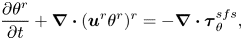 \begin{gather} \frac{ \partial \theta^{r}}{ \partial t}+ \boldsymbol{\nabla} \boldsymbol{\cdot} (\boldsymbol{u}^{r} \theta^{r})^{r} ={-} \boldsymbol{\nabla} \boldsymbol{\cdot} {\boldsymbol{\tau}}_{\theta}^{sfs}, \end{gather}
 \begin{gather} \boldsymbol{\nabla} \boldsymbol{\cdot}\boldsymbol{u}^{r} = 0, \end{gather}
where LES resolved-scale variables are indicated with superscript  $r$,
$r$,  $\boldsymbol {u}^{r}$ is the resolved velocity vector,
  $p^{*}$ is the effective resolved fluctuating pressure (see below) and
  $\theta ^{r}$ is the resolved potential temperature. The sub-filter-scale (SFS) ‘stress’ tensor
  ${\boldsymbol {\tau }}^{sfs}=( \boldsymbol {u}^{r}\boldsymbol {u}^{s}+ \boldsymbol {u}^{s}\boldsymbol {u}^{r}+\boldsymbol {u}^{s}\boldsymbol {u}^{s})^{r}$ and temperature flux vector
  ${\boldsymbol \tau }^{sfs}_{\theta }=( \theta ^{r}\boldsymbol {u}^{s}+ \theta ^{s}\boldsymbol {u}^{r}+\theta ^{s}\boldsymbol {u}^{s})^{r}$ must be modelled, where superscript
  $s$ indicates SFS variables. Typically,
  ${\boldsymbol {\tau }}^{sfs}$ is separated into its isotropic and deviatoric parts, with its isotropic part included in
  $p^{*}$ (see below) and its deviatoric part
  $\boldsymbol {\tau }^{sfs}_a$ modelled using the one-equation eddy viscosity closure described in Moeng (Reference Moeng1984) (see also Deardorff Reference Deardorff1980; Sullivan, McWilliams & Moeng Reference Sullivan, McWilliams and Moeng1996; Khanna & Brasseur Reference Khanna and Brasseur1997):
 \begin{equation} \boldsymbol{\tau}_a^{sfs}={-}2\nu_T\boldsymbol{\mathsf{s}}^{r}, \quad \nu_T=C_kl\sqrt{e}, \quad \varDelta=(\varDelta_x,\varDelta_y,\varDelta_z)^{1/3}, \quad C_k=0.08, \end{equation}
where
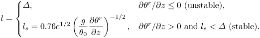 \begin{equation} l = \left\{ \begin{array}{@{}ll} \varDelta, & \partial\theta^{r}/ \partial z \leq 0 \text{ (unstable)}, \\ l_s=0.76e^{1/2}\left(\dfrac{g}{\theta_0}\dfrac{ \partial\theta^{r}}{ \partial z}\right)^{{-}1/2}, & \partial\theta^{r}/ \partial z > 0 \text{ and } l_s<\varDelta \text{ (stable)}. \end{array} \right. \end{equation}
Here  $\boldsymbol{\mathsf{s}}^{r}$ is the resolved strain-rate tensor,
  $\varDelta _{x,y,z}$ are the cell dimensions for uniform hexahedral grid cells,
  $l$ and
  $\varDelta$ represent the SFS and grid length scales, respectively, and
  $e$ is the ‘SFS turbulent kinetic energy’, solved using a prognostic equation as in Moeng (Reference Moeng1984). In all simulations
  $C_k=0.08$. The SFS temperature flux vector
  $\boldsymbol {\tau }_{\theta }^{sfs}$ is also modelled with an eddy diffusivity closure (Deardorff Reference Deardorff1980; Moeng Reference Moeng1984):
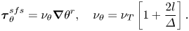 \begin{equation} {\boldsymbol \tau}_{\theta}^{sfs}=\nu_{\theta} \boldsymbol{\nabla}\theta^{r}, \quad \nu_{\theta}=\nu_T\left[1 + \frac{2l}{\varDelta}\right]. \end{equation}
 The momentum equation (2.1) adopts the Boussinesq approximation for gravitational force with the background state variables  $\rho _0$ and
  $\theta _0$ taken as the initial surface values. The local resolved pressure
  $p^{r}=p^{r\,\prime }+P$ is separated into ensemble mean (
 $P$) and fluctuating parts, with the fluctuating part included in effective pressure,
  $p^{*}=p^{r\,\prime }-({\rho _0}/{3})\, \textrm {tr} \{ \boldsymbol {\tau }^{sfs} \}$. Mean pressure gradient
  $\boldsymbol {\nabla } P$ is written in terms of a specified ‘geostrophic wind’ vector
  $\boldsymbol {V}_g$, defined through the Ekman balance between pressure and Coriolis force:
 \begin{equation} \boldsymbol{\nabla}_h P\equiv \rho_0 \,\boldsymbol{f}\times \boldsymbol{V}_g, \end{equation}
where  $\boldsymbol {f}=f\hat {\boldsymbol {e}}_z$ is twice the projected Earth rotation-rate vector. In the canonical ABL,
  $\boldsymbol {V}_g$ and
  ${ \boldsymbol {\nabla }} P$ are horizontal and
  $\boldsymbol {V}_g$ describes the mesoscale wind, which is set to a nominal value of
  $10\ \textrm {m}\,\textrm {s}^{-1}$ for this study. In our simulations the Coriolis parameter
  $f\equiv |\,\boldsymbol {f}|$ is set to
  $10^{-4}\ \textrm {s}^{-1}$ as representative of the mid-latitudes. The specification of
  $\boldsymbol {V}_g$ in concert with surface heat flux
  $Q_0$ establishes the stability state
  $-z_i/L$ of the boundary layer after reaching quasi-equilibrium.
2.1.1. The quasi-equilibrium state
The ABL is capped by a stabilizing inversion layer in potential temperature, established in part through specification of the initial condition in the potential temperature field. The initial potential temperature profile is constant up to the initial capping inversion height  $z_{i_o}$ and increases from
  $z_{i_o}$ to the top of the computational domain with constant slope. The rate at which the capping inversion depth grows with time (
 $\textrm {d}z_i/\textrm {d}t$) increases with surface heat flux
  $Q_0$, leading to concerns with potential influence on stationarity, and therefore equilibrium. In addition, if
  $z_i$ were to increase to
  ${\sim }2/3$ the domain height, it would become necessary to increase the extent of the vertical domain and modify the grid, which might impact subtle transitions in ABL structure. To minimize these concerns, the initial capping inversion strength, quantified by the vertical gradient in mean potential temperature within the capping inversion layer,
  $[\textrm {d}\theta ^{r}/\textrm {d}z]_{CI}$, was carefully chosen to minimize the rate of growth in
  $z_i$ at the highest
  $Q_0$ (and
  $-z_i/L$) while remaining consistent with observations of capping inversion strengths in the daytime atmosphere. In the current study, the magnitude of
  $[ \textrm {d}\theta ^{r}/\textrm {d}z ]_{CI}$ averaged over the capping inversion layer was
  ${\simeq }87\ \textrm {K}\,\textrm {km}^{-1}$ with a standard deviation of
  $37\ \textrm {K}\,\textrm {km}^{-1}$ over 14 simulations (table 1). For comparison, the LES study of Sullivan & Patton (Reference Sullivan and Patton2011) adopted a capping inversion temperature gradient of
  $\simeq 80\ \textrm {K}\,\textrm {km}^{-1}$. To estimate realistic ranges of capping inversion strengths, we analysed data from the open literature (Sorbjan Reference Sorbjan1996; Sullivan et al. Reference Sullivan, Moeng, Stevens, Lenschow and Mayor1998; Hennemuth & Lammert Reference Hennemuth and Lammert2006) as well as from a database collected from aircraft flights in Indiana (Davis Reference Davis2017). Using these, we estimated the capping inversion strengths in the daytime ABL to lie between
  $9.8\ \textrm {K}\,\textrm {km}^{-1}$ and
  $120\ \textrm {K}\,\textrm {km}^{-1}$ with a mean of
  $56\ \textrm {K}\,\textrm {km}^{-1}$ and standard deviation of
  $40\ \textrm {K}\,\textrm {km}^{-1}$, indicating that the capping inversion strengths in our LES experiments are within observational ranges. Additionally, the depths of capping inversions in our LES were in the range of those analysed from available field data (see Grabon et al. Reference Grabon, Davis, Kiemle and Ehret2010).
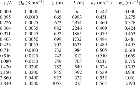
Table 1. Simulation parameters over the quasi-stationary analysis periods.
In figure 1 we plot the ratio of capping-inversion-growth velocity to buoyancy-driven mixed layer velocity scale  $w_*$ for the capping inversion strength
  $[ \textrm {d}\theta ^{r}/\textrm {d}z ]_{CI}$ adopted in our computations at our highest
  $Q_0$ (
 $-z_i/L=3.84$), demonstrating that the worst case
  $\textrm {d}z_i/\textrm {d}t$ is well over two orders of magnitude smaller than the dominant characteristic velocity scale (consistent with Sullivan & Patton (Reference Sullivan and Patton2011)), thus maintaining quasi-stationarity. The fully developed quasi-equilibrium period for analysis was chosen from the simulation window over which the friction velocity (
 $u_*$), buoyancy velocity scale (
 $w_*$) as well as the net mass flow rate through the domain become nearly constant with time. This quasi-equilibrium is realized after
  ${\sim }200$ eddy turnover times,
  $\tau _u\equiv z_i/u_*$. The time periods over which statistics were calculated in this analysis varied between
  $60\tau _u$ and
  $80\tau _u$ for the different
  $-z_i/L$.
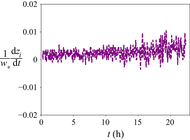
Figure 1. Time evolution of the ratio of capping-inversion-growth velocity to the buoyancy-driven mixed layer velocity scale at the highest  $-z_i/L\simeq 3.84$ for the chosen initial capping inversion strength.
The dynamical system was discretized within a rectangular computational domain  $5\ \text {km} \times 5\ \text {km} \times 2\ \text {km}$ using a uniformly spaced geometric grid of dimension
  $324 \times 324 \times 96$. The pseudo-spectral algorithm was applied in the horizontal with periodic boundary conditions; second-order finite differencing was applied in the vertical on a staggered grid. Dealiasing by truncation in the horizontal using the 2/3 rule creates an effective grid of
  $216 \times 216 \times 96$ points with cell aspect ratio of
  ${\simeq }1$ on which the resolved scales evolve. Note that effective grid resolution (as opposed to geometric grid resolution) is quoted in all figures. A series of
  $14$ simulations were carried out to equilibrium with systematically varying surface heat flux for fixed geostrophic wind velocity magnitude of
  $10\ \textrm {m}\,\textrm {s}^{-1}$ and direction (aligned with
  $x$). Over the periods of data collection, the vertical extent of the domain is
  $2z_i$–
 $3z_i$, so that the boundary layer was resolved in the vertical with 31–51 points and the surface layer with 8–12 points. Time advance was performed using third-order Runge–Kutta integration.
For each simulation, the initial potential temperature distribution was constant in  $z$ up to the initial capping inversion layer of thickness
  ${\simeq }200\ \text {m}$ centred at
  $z\simeq 640\ \text {m}$ with temperature difference of 30 K (
 $[\textrm {d}\theta ^{r}/\textrm {d}z]_{CI}=0.144\ \textrm {K}\,\textrm {m}^{-1}$). Above this layer, the initial vertical temperature gradient was set to
  $0.003\ \textrm {K}\,\textrm {m}^{-1}$. On the upper boundary, the mean temperature gradient is fixed at the initial value and the vertical gradients of the horizontal velocity components, the SFS viscosity and the vertical velocity were all fixed at zero. On the lower surface, the temperature flux
  $Q_0=\langle w\theta \rangle _0$ was prescribed at the
  $14$ values given in table 1. A lower boundary condition on total surface fluctuating shear stress vector was applied similarly to the nonlinear model described in Moeng (Reference Moeng1984), which was also applied in the studies by Khanna & Brasseur (Reference Khanna and Brasseur1997, Reference Khanna and Brasseur1998), Brasseur & Wei (Reference Brasseur and Wei2010) and Sullivan & Patton (Reference Sullivan and Patton2011). The surface stress model introduces a roughness parameter
  $z_0$ in a modelled relationship for the ratio of mean horizontal velocity magnitude at the first grid level
  $U_1$ to the friction velocity
  $u_*=|\langle \boldsymbol {u}_hw \rangle |^{1/2}_0$. This modelled relationship for
  $U_1/u_*$ is based on a continuous function of
  $z/z_0$ given by the empirical form of Monin–Obukhov law-of-the-wall (LOTW) scaling developed by Paulson (Reference Paulson1970) for the surface layer. The roughness parameter
  $z_0$ is set to
  $0.16\ \text {m}$ in our study.
2.1.2. LES grid design and overshoot
Grid design for LES is complicated by the interaction between resolution, grid cell aspect ratio and SFS parametrization. Specifically, an issue inherent to LES of the rough-surface ABL is the problem of the near-surface ‘overshoot’, an overprediction of mean velocity gradient at the first few LES grid cells adjacent to the surface. The overshoot is characterized as a peak in the vertical mean velocity gradient after normalization by inertial LOTW scaling in  $z$ (see Piomelli (Reference Piomelli2008) and Brasseur & Wei (Reference Brasseur and Wei2010, BW10), and references therein, for detailed discussions of this issue). This long-standing problem with LES prediction has been diagnosed by BW10 as arising from the inconsistency between the inertia dominance requirement in the LOTW scaling argument for the inertial surface layer and non-physical frictional content within the SFS stress model. The strength of the spurious frictional content depends on the design of the grid (specifically, vertical resolution and grid cell aspect ratio). The base effective grid (i.e. after dealiasing in the horizontal) of dimension
  $216 \times 216 \times 96$ used in this study was designed to eliminate this spurious overshoot after following through a systematic procedure involving numerous LES of different grids (nearly
  $80$ simulations across the various
  $-z_i/L$). In appendix A.1 we describe the application of the BW10 framework to systematically remove the overshoot from all simulations. This analysis is extended in appendix A.2 to the design and application of grids to study impacts of varying resolution.
In total, 14 simulations (figure 2 and table 1) were carried out to quasi-equilibrium and analysed with instability state parameter  $-z_i/L$ from
  $0$ to
  $3.84$ corresponding to
  $Q_0$ from
  $0$ to
  $0.050\ \textrm {K}\,\textrm {m}\,\textrm {s}^{-1}$ with fixed geostrophic wind speed of
  $10\ \textrm {m}\,\textrm {s}^{-1}$. The stability parameter
  $-z_i/L$ varies approximately linearly with
  $Q_0$ (figure 2a), largely due to surface friction velocity
  $u_*$ and capping inversion height
  $z_i$ varying relatively little with
  $-z_i/L$ (figure 2b). In contrast, the Obukhov length
  $L$ and buoyancy velocity scale
  $w_*\equiv ( gQ_0z_i/\theta _0 )^{1/3}$ vary approximately as
  $1/Q_0$ and
  $Q_0^{1/3}$, respectively.
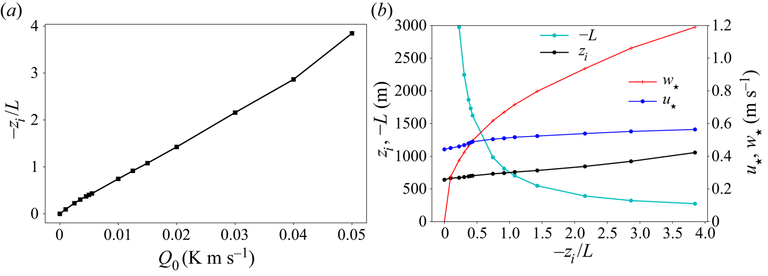
Figure 2. (a) Variation of instability parameter with surface heat flux. (b) Variation of simulation parameters with instability state,  $-z_i/L$.
2.2. Analytical methods applied to the LES data
To study transitions in the structure of the most energy-dominant turbulence motions within the ABL, we quantify two-point correlations and coherence lengths. These converged statistics are estimated by leveraging horizontal homogeneity and quasi-stationarity to average over horizontal planes and the  ${\sim }70\tau _u$ analysis window over which the capping inversion depth
  $z_i$ grew by
  ${\sim }10\,\%$ for the most convective instability state (
 $-z_i/L = 3.84$), less for less unstable states. Some second- and third-order moments are also quantified to characterize variances, covariances and terms in the budget equations for turbulent kinetic energy. Unless otherwise specified, all statistics are calculated with
  $x$ and
  $y$ rotated to align with the mean velocity vector in that horizontal plane such that the rotated coordinate system
  $(x^{r}_1, x^{r}_2, x_3) \equiv (x_{rot}(z), y_{rot}(z), z)$ varies with
  $z$.
$z$.
The two-point velocity–velocity correlation on horizontal planes in rotated coordinates is given by
 \begin{equation} {R}_{ij,k}(r_k,z)=\langle u^{r}_i(\boldsymbol{x}^{r}_h,z)u^{r}_j(\boldsymbol{x}^{r}_h+r_k\boldsymbol{e}^{r}_k,z) \rangle, \end{equation}
where  $u^{r}_i$ are the fluctuating velocity components in the rotated coordinates and there is no sum on
  $k$. Homogeneity in the horizontal implies that the correlation is independent of starting point
  $\boldsymbol {x}^{r}_h$ on the horizontal plane and that the ensemble averages can be replaced by averages over horizontal planes at fixed z. In (2.7)
  $r_k$ is restricted to the horizontal plane
  $(k = 1,2)$, all in the rotated coordinates. Thus,
  $R_{ij,k}$ depends only on
  $z$, in addition to
  $r_k$. The two-point velocity–velocity correlation in the
  $z$ direction is given by
 \begin{equation} {R}_{ij,3}(r_3,z_0)=\langle u_i(\boldsymbol{x}_h,z_0)u_j(\boldsymbol{x}_h,z_0+r_3) \rangle, \end{equation}
where  $u_i$ and
  $\boldsymbol {x}_h \equiv (x_1, x_2)$ are the fluctuating velocity components and horizontal location in unrotated coordinates. In the inhomogeneous
  $z$ direction, the two-point correlation depends on the starting point,
  $z_0$ (chosen as
  $0.1z_i$) and
  $r_3=z-z_0$ is the distance in the vertical direction. In our analysis, the angle brackets in (2.7) and (2.8) imply averaging both in space over the horizontal
  $z$ planes and in time over at least
  $60$ integral time scales
  $\tau _u$ during the quasi-equilibrium period.
The corresponding integral scales are given by
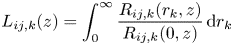 \begin{equation} {L}_{ij,k}(z) =\int_0^{\infty} \frac{R_{ij,k}(r_k,z)}{R_{ij,k}(0,z)}\,\textrm{d}r_k \end{equation}
on a horizontal plane and by
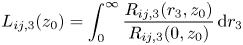 \begin{equation} {L}_{ij,3}(z_0) =\int_0^{\infty} \frac{R_{ij,3}(r_3,z_0)}{R_{ij,3}(0,z_0)}\,\textrm{d}r_3 \end{equation}
in the vertical direction. The integral scale in the vertical is estimated using non-rotated coordinates. We have confirmed that the vertical integral scales are mostly insensitive to the rotation of the horizontal coordinates. In practice, the integral in (2.9) is calculated using Fourier decomposition in the horizontal, which effectively ends the integration of the two-point correlation at half the horizontal domain width. To calculate (2.10), the integral extends to the capping inversion,  $z_i$. Further discussion on the calculation of integrals is given in § 7 and appendix A.3.
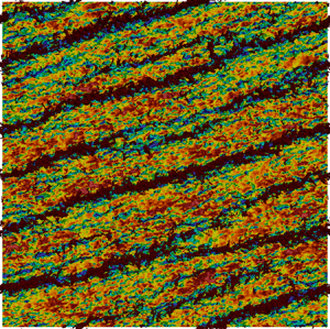
3. Overview of transition in the ABL turbulence structure from neutral to moderately convective
The changes in structure of energy-dominant atmospheric turbulence eddies in the canonical daytime ABL as a function of instability parameter  $-z_i/L$ are difficult to quantify systematically in the field, especially when the data used must be restricted to quasi-equilibrium periods. A major advantage of LES is the ability to more accurately approximate the canonical equilibrium ABL state with statistical structure that is dependent only on
  $-z_i/L$. Furthermore, with LES we can simultaneously quantify and visualize details of four-dimensional large-eddy motions through highly controlled variation in atmospheric stability at levels of refinement not possible in the field. Of particular interest here are the subtle (and not so subtle) changes in horizontal and vertical characteristic coherence length scales associated with progressive increases in surface heating from the neutral ABL with fixed geostrophic (i.e. mesoscale) winds.
In this section, we describe in broad terms our analysis of the rich transition in the energy-dominant coherent structure of the ABL with increasing instability from neutral to a roll-dominated moderately convective state in the range  $-z_i/L\sim 0\text {--}4$. In subsequent sections we elaborate on specific characteristics in the transitions in turbulence structure that define ‘regimes of transition’, including a ‘critical stability regime’ where small changes from the near-neutral stability create major changes in ABL structure (§ 4) and a ‘maximum coherence regime’ associated with large-scale atmospheric rolls (§ 5), both sandwiched between neutral and moderately convective states (§ 6).
3.1. Trends in coherence lengths
The production of streamwise velocity fluctuations originates statistically from the interaction between mean shear and Reynolds shear stress. Furthermore, stability theory (Lilly Reference Lilly1966; Brown Reference Brown1980) and studies of homogeneous turbulent shear flow (Lee et al. Reference Lee, Kim and Moin1990; Brasseur & Wang Reference Brasseur and Wang1992; Brasseur & Lin Reference Brasseur and Lin2005) show that streamwise coherence is created by the dynamical interactions between mean shear rate  $S$ and the underlying turbulence fluctuations, an effect that strengthens with normalized shear rate,
  $S\tau _u$. Therefore, one anticipates that the streamwise coherence length of streamwise velocity fluctuations (
 $L_{11,1}$) in the surface layer will be highest in the purely shear-dominated neutral state (
 $-z_i/L = 0$) and that any addition of surface heating (i.e.
  $-z_i/L > 0$) will interfere with this mechanism and reduce streamwise coherence. If this is the case, then the streamwise coherence length of streamwise velocity fluctuations,
  $L_{11,1}$, should decrease monotonically with increasing
  $-z_i/L$ from the neutral state.
Surprisingly, this turns out not to be the case, as shown in figure 3(a), where  $L_{11,1}$ is plotted against
  $-z_i/L$ at different distances from the surface. Our simulations predict that streamwise coherence lengths of streamwise fluctuations
  $u^{\prime }$ actually increase with increasing
  $-z_i/L$ as surface heat flux
  $Q_0$ is added to a previously unheated neutral canonical ABL. This response is strong and occurs with small increases in
  $Q_0$ and instability state, and is observed through the entire boundary layer from near the surface (
 $z/z_i=0.1$) to near the capping inversion (
 $z/z_i=0.7$). The anticipated reduction in streamwise coherence length with increase in
  $-z_i/L$ does occur, but not until
  $L_{11,1}$ has first increased by over a factor of 2 everywhere. The doubling of horizontal coherence length
  $L_{11,1}$ initiates at
  $-z_i/L \simeq 0.30$ and peaks at
  $-z_i/L = 0.433$ after the addition of very small levels of surface heating (from figure 2(a) and table 1,
  $Q_0 = 0.0055\ \textrm {K}\,\textrm {m}\,\textrm {s}^{-1}$ at
  $-z_i/L = 0.433$). The sudden increase in
  $L_{11,1}$ from
  $-z_i/L \simeq 0.30$ and
  $\simeq 0.43$ is followed by the expected monotonic decrease.
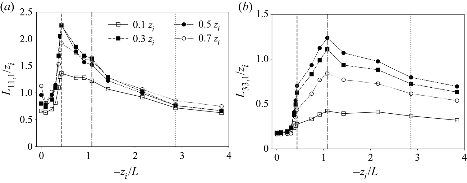
Figure 3. Variation of streamwise coherence lengths of (a) streamwise velocity fluctuations ( $L_{11,1}$) and (b) vertical velocity fluctuations (
 $L_{33,1}$) with the global instability parameter
  $-z_i/L$. Each curve corresponds to fixed height within the boundary layer as indicated. The three vertical lines in each panel correspond to the following important transition states:
  $-z_i/L=0.433$ (dashed),
  $-z_i/L=1.080$ (dot-dashed) and
  $-z_i/L=2.86$ (dotted).
A similar trend is also observed in the streamwise coherence length of vertical velocity fluctuations  ${w^{\prime }}$ (
 $L_{33,1}$), but with significant differences (figure 3b). In particular, a sudden increase in coherence length occurs at
  $-z_i/L=0.433$ for
  $L_{33,1}$ as it does in
  $L_{11,1}$, albeit with less variation when
  $-z_i/L\leq 0.304$. Also, the variation is much less pronounced at
  $z_i/z=0.1$, where vertical velocity fluctuations are damped at all
  $-z_i/L$. More importantly, however, whereas
  $L_{11,1}$ decreases monotonically when
  $-z_i/L$ increases above the critical value of
  $0.433$,
  $L_{33,1}$ continues to increase to a peak at
  $-z_i/L=1.08$, after which it decreases monotonically. It is interesting that the normalized horizontal coherence lengths at the highest values of
  $-z_i/L$ simulated are all roughly in the range
  $0.6z_{i}\text {--}0.7z_i$ for both horizontal and vertical turbulence fluctuations at all levels in the ABL, with the exception of
  $L_{33,1}$ at the highly damped location
  $z/z_i = 0.1$. Also note that, whereas both
  $L_{11,1}$ and
  $L_{33,1}$ individually increase to a peak coherence length, the total relative increase in streamwise coherence length is, overall, much larger for vertical fluctuating velocity due to its smaller values in the neutral regime. These observations will be discussed in more detail in § 4, where we analyse the existence of a ‘critical’ instability at
  $-z_i/L\simeq 0.43$. This intriguing and non-monotonic transition in the coherence lengths of the energy-containing turbulent velocity fluctuations (
 $L_{11,1}$ and
  $L_{33,1}$) also manifests in the organization and overall structure of the energy-dominant turbulent eddies as
  $-z_i/L$ increases, thereby suggesting a complex interplay between energy-containing buoyancy and shear-driven turbulent motions.
In appendices A.2 and A.3 we describe an analysis of the impacts of grid resolution and horizontal domain resolution, respectively, on the results presented in figure 3. Overall, we find that, although resolution and domain size impacts are not negligible, the key features identified here are accentuated with increase in resolution or horizontal domain size (on appropriately designed grids). These issues are further discussed in § 7.
3.2. Trends in single-point statistics
Figure 4 shows the changes in select terms in the Reynolds stress tensor and their budget equations with systematic variation in stability state. In general, the variances and covariances show less dramatic variations with  $-z_i/L$ (figure 4) as compared to the relative changes in streamwise coherence length with
  $-z_i/L$ (figure 3). However, all the different single-point statistical metrics show perceptible changes occurring at
  $-z_i/L=0.433$ (highlighted by the dashed vertical line), indicating a critical transition at this instability state. For example, the streamwise fluctuating velocity variance (figure 4a) increases to a peak at
  $-z_i/L=0.433$ over the entire boundary layer before gradually decreasing to smaller values at higher
  $-z_i/L$, not dissimilar to the variation of
  $L_{11,1}$ with
  $-z_i/L$ (figure 3a). The transition in streamwise variance production near the surface (figure 4e) also shows a peak at
  $-z_i/L=0.433$ followed by a nearly linear decrease.
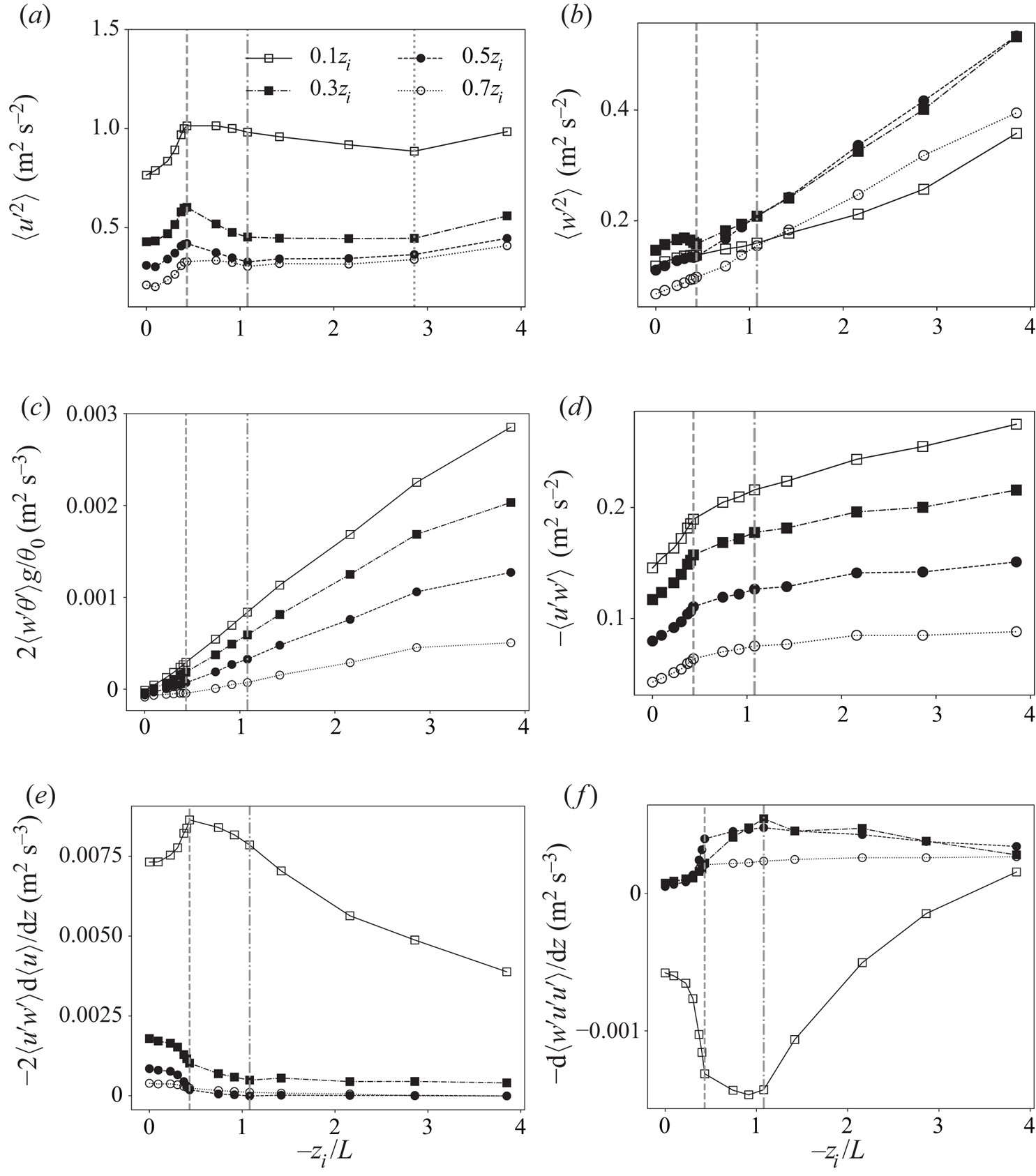
Figure 4. Transition of turbulence statistics with the global instability parameter  $-z_i/L$ at fixed vertical locations in the ABL, as specified by the line types and symbols defined in panel (a): (a) streamwise velocity variance,
  $\langle {u^{\prime }}^{2} \rangle$; (b) vertical velocity variance,
  $\langle {w^{\prime }}^{2} \rangle$; (c) rate of production of vertical velocity variance by buoyancy force (proportional to vertical potential temperature flux),
  $2\langle w^{\prime }\theta ^{\prime }\rangle g/\theta _0$; (d) vertical turbulent momentum flux,
  $\langle u^{\prime }w^{\prime } \rangle$; (e) shear production rate of streamwise velocity variance,
  $-2\langle u^{\prime }w^{\prime }\rangle ({\textrm {d}\langle u\rangle }/{\textrm {d}z})$; and (f) time rate of change of horizontal velocity variance due to vertical turbulent transport,
  $-({\textrm {d}\langle w^{\prime }u^{\prime }u^{\prime }\rangle }/{\textrm {d}z})$. Here (
 $u^{\prime },v^{\prime },{w^{\prime }}$) are the fluctuating parts of resolved velocity in a local frame of reference with
  $x$ aligned with the mean velocity vector at that height,
  $z$. The two (three) vertical lines correspond to the key transition states:
  $-z_i/L=0.433$ (dashed),
  $-z_i/L=1.080$ (dot-dashed) and
  $-z_i/L=2.86$ (dotted).
Away from the surface, the magnitude of shear-induced production rate (figure 4e) decreases while its transition with  $-z_i/L$ shows a sharp decrease near
  $-z_i/L=0.433$ before asymptoting at the more unstable states. The lack of a peak in shear-induced streamwise variance production away from the surface does not support the observed peaks in the streamwise variance at these heights (figure 4a). To explain this, consider vertical turbulent transport in the streamwise variance budget (figure 4f). This figure shows that streamwise velocity fluctuations generated closer to the surface are transported to the mixed layer, on average, by vertical velocity fluctuations. The extent of this transport grows sharply around
  $-z_i/L \simeq 0.43$ and peaks at
  $-z_i/L \simeq 1.08$. These observations suggest that the streamwise variance structure across the entire ABL is affected by a combination of production from shear closer to the surface and transport of turbulence by buoyancy-driven vertical velocity fluctuations away from the surface, in a manner dependent on the stability state parameter
  $-z_i/L$. Furthermore, the non-monotonic variation of shear-driven streamwise variance with
  $-z_i/L$, in spite of constant geostrophic wind forcing, is partially a consequence of buoyancy and shear-rate contributions to pressure–strain-rate correlation.
Both vertical velocity variance (figure 4b) and its production from buoyancy (figure 4c) grow nearly linearly with  $-z_i/L$ throughout the ABL, a trend consistent with the near-linear increase in surface heat flux,
  $Q_0=\langle w^{\prime }\theta ^{\prime } \rangle _0$, which is specified at the surface to control the changes in global stability parameter in our computations. However, we observe slight decreases in
  $\langle w'^{2} \rangle$ near
  $-z_i/L=0.433$ in the mixed layer region that can be attributed to mechanisms other than production. The transition in Reynolds stress
  $\langle u'w' \rangle$ with
  $-z_i/L$ (figure 4d), whose evolution is tied to the vertical variance through the mean gradient production term
  $\langle w'^{2} \rangle \partial \langle u \rangle /\partial z$, also grows monotonically with
  $-z_i/L$ similar to
  $\langle w'^{2} \rangle$, but with sharper changes around
  $-z_i/L = 0.433$.
In summary, almost all of the statistical measures shown in figure 4 display intriguing transition around  $-z_i/L = 0.433$ although the specific details differ among the variables. The mechanics of this transition depends not only on turbulence production, but also on turbulence transport processes driven by buoyancy forces, especially around
  $-z_i/L = 1.08$. These observations suggest that the interesting responses to increasing
  $-z_i/L$ in the two-point statistical measures are dynamically correlated with the responses in single-point statistics (figure 4). This is particularly true of the streamwise coherence lengths of streamwise velocity fluctuations (figure 3a) and vertical velocity fluctuations (figure 3b), which peak at
  $-z_i/L = 0.433$ and
  $-z_i/L=1.08$, respectively.
4. A critical stability state ( $-z_i/L \approx 0.43$)

Figure 3 suggests a minor response to surface heat flux up to  $Q_0\approx 0.004\ \textrm {K}\,\textrm {m}\,\textrm {s}^{-1}$, which is only 1 %–2 % of the average peak midday temperature flux of roughly
  $0.25\ \textrm {K}\,\textrm {m}\,\textrm {s}^{-1}$ (Wyngaard Reference Wyngaard2010) and corresponds to a very low stability state parameter
  $-z_i/L\approx 0.30$. Beyond this state, a dramatic change in integral-scale turbulence eddying structure takes place up to
  $-z_i/L=0.433$, associated with a sudden increase in the streamwise coherence lengths
  $L_{11,1}$ and
  $L_{33,1}$ when
  $Q_0$ is only
  $0.0055\ \textrm {K}\,\textrm {m}\,\textrm {s}^{-1}$ (table 1). Interestingly, the critical transition state of
  $-z_i/L=0.433$ occurs when
  $u_*/w_*\sim O(1)$ (figure 2), when the intensity of buoyancy-driven and shear-driven turbulent kinetic energy coincides. Here, we analyse this sudden change in ABL turbulence structure at stability states previously thought to be near-neutral (Khanna & Brasseur Reference Khanna and Brasseur1998).
4.1. The existence of a critical transition in statistical coherence
We argue that the extreme sensitivity shown in figure 3 between very small increases in heating rate and ABL turbulence structure suggests critical transition dynamics. The streamwise coherence lengths of both streamwise and vertical turbulence velocity fluctuations ( $L_{11,1}$ and
  $L_{33,1}$) more than double across the ABL with extremely small increases in instability state parameter at
  $-z_i/L$ values considered to be ‘near-neutral’. In the mixed layer, in particular,
  $L_{11,1}$ increases from
  $0.7z_i$ to
  $2.1z_i$, a factor of 3 increase, while
  $L_{33,1}$ increases from roughly
  $0.16z_i$ to
  $0.70z_i$, over a four-fold growth from neutral to critical states. These dramatic increases in coherence lengths at critical transition occur with much smaller relative increases in horizontal variances (figures 4a and 4b).
Figure 5 shows that, at the critical stability state, the entire ABL structure changes dramatically. Here we plot the horizontal integral scales of horizontal (figure 5a) and vertical velocity (figure 5b) fluctuations at fixed stability states across the boundary layer. In the current discussion, we focus on the transition between the blue and red curves. The blue curves indicate relatively minor changes in horizontal integral-scale structure in the near-neutral precritical (subcritical) states, culminating with the line with symbols at  $-z_i/L=0.304$ just before the sudden transition in structure represented by the red curves. Whereas
  $L_{11,1}$ changes relatively little within the boundary layer in the precritical (subcritical) period,
  $L_{33,1}$ remains virtually unchanged. However, with very small changes in stability state parameter from
  $-z_i/L =0.304$ (blue symbolled curve) to the critical state
  $-z_i/L=0.433$ (red symbolled curve), the streamwise integral scales of both horizontal and vertical velocity fluctuations increase sharply over the entire boundary layer. The value of
  $L_{11,1}/z_i$ changes from roughly 1 to over 2 in the lower mixed layer (
 $z/z_i \simeq 0.34$), while
  $L_{33,1}/z_i$ increases from a small fraction to order
  $1$ in the mid mixed layer (
 $z/z_i \simeq 0.44$). As in figure 3, figure 5 shows that
  $L_{11,1}$ reaches a sharp peak at the critical state (
 $-z_i/L\simeq 0.433$) while
  $L_{33,1}$ continues to grow more gradually beyond an initial large jump at the critical state to a peak at
  $-z_i/L\simeq 1.08$, a post-critical process that will be discussed in § 5 in context with the formation of large-scale rolls. Interestingly, the sudden transition in
  $L_{11,1}$ and
  $L_{33,1}$ at the critical state is much stronger in the mixed layer than either near the ground or nearer to the capping inversion, where blockage in the vertical causes reductions in correlation lengths.
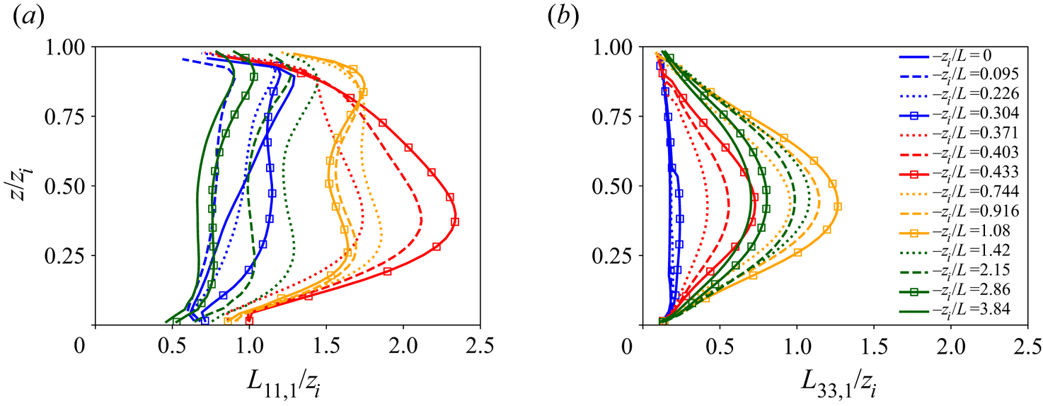
Figure 5. Transition in streamwise coherence lengths over the vertical extent of the ABL at fixed instability states,  $-z_i/L$. (a) Streamwise coherence length of fluctuating horizontal velocity (
 $L_{11,1}$). (b) Streamwise coherence length of vertical fluctuating velocity (
 $L_{33,1}$). The line colours are chosen to be consistent with discussions in the text on the changes in ABL coherence structure surrounding special stability states: blue indicates subcritical stability states near neutral, while red indicates the rapid transition from
  $-z_i/L=0.304$ (blue line with symbols) to the critical state
  $-z_i/L=0.433$ (red line with symbols). Yellow lines indicate the transition from the critical state to the ‘maximum coherence state’
  $-z_i/L=1.08$ dominated by large-scale rolls (yellow line with symbols), followed by green lines indicating further transition to the ‘moderately convective’ states when
  $-z_i/L\gtrsim 2.86$ (green line with symbols).
Figure 5 shows a mild subcritical response of horizontal coherence length to slight increases in surface heating, but only in the streamwise, not the vertical, velocity fluctuations. However, in the transition to the critical state (red curves), the entire streamwise coherence of the boundary layer changes dramatically, with maximum streamwise coherence lengths peaking in the lower mixed layer for horizontal velocity fluctuations ( $L_{11,1}$) and in the mixed layer for vertical fluctuations (
 $L_{33,1}$). This sudden change at the critical state is primarily in the coherence structure of the ABL with relatively minor impact on fluctuation levels (variances in figures 4(a) and 4(b) show at most
  $10\,\%$ change).
Such abrupt restructuring of the entire ABL structure suggests the initiation of a global instability from the interaction between shear-driven turbulent motions and low-level buoyancy-driven motions. Additionally, in the transition from subcritical ( $-z_i/L \lesssim 0.304$) to supercritical (
 $-z_i/L \gtrsim 0.433$), streamwise coherence lengths change from being roughly uniform over the ABL to peaking in the mixed layer away from the surface (figure 5) – suggesting a dramatically altered dynamical state through sudden linking of the lower and mid boundary layer.
To quantify this linkage, we plot in figure 6 the coherence lengths in the vertical direction from two-point correlations in  $z$ referenced to
  $z/z_i=0.1$ (integral length scales are therefore normalized on
  $0.9z_i$). Interestingly, whereas in the neutral state the horizontal and vertical velocity fluctuations have the same vertical coherence length (roughly
  $0.2z_i$), these vertical scales diverge with the addition of low levels of surface heat flux in the subcritical state. In particular, the vertical coherence length of horizontal fluctuations (
 $L_{11,3}$) increases by
  $56\,\%$ at the critical state while the average vertical coherence length of vertical velocity concentrations changes little. As the streaks suddenly extend in the horizontal by a factor of 3 in the lower mixed layer, they fatten in the vertical by roughly
  $50\,\%$. At the same time, the concentrations of vertical velocity do not change in scale in the vertical, but extend in the horizontal by over a factor of 4 (!) with slight increase in surface heat flux. We will show in the next section that, as
  $-z_i/L$ continues to increase from critical, the vertical scale of horizontal fluctuations decreases post-critical while that of vertical velocity initiates a monotonic increase until they match.

Figure 6. Transitions of vertical coherence lengths with instability parameter  $-z_i/L$ calculated vertically from level
  $z=0.1z_i$. The solid, dashed and dotted curves correspond to vertical coherence length of horizontal, spanwise and vertical velocity fluctuations, respectively. The three vertical lines correspond to transition states:
  $-z_i/L=0.433$ (dashed),
  $-z_i/L=1.080$ (dot-dashed) and
  $-z_i/L=2.86$ (dotted).
We conclude that the initiation of the dramatic transition in ABL structure occurs primarily in the streamwise coherence of both horizontal and vertical velocity fluctuations in the lower (horizontal) and mid (vertical) surface layer, with a fattening of the horizontal fluctuations (streaks) in the vertical. The implication is that the critical state corresponds to an increase in communication between the lower and mid ABL through the stimulation of an overlap in the lower-to-mid mixed layer between concentrations of horizontal and vertical fluctuations. This takes place as the horizontal coherence lengths of both increase dramatically – without the stimulation of thermals in the vertical. However, whereas transition to the critical state does not stimulate a change in vertical coherence of vertical fluctuations,  $L_{33,3}$, it does initiate a monotonic growth (of
  $L_{33,3}$ discussed in §§ 5 and 6). It appears that the dramatic restructuring of the entire boundary layer around the critical transition state is not due to a sudden creation of non-local communication between the lower and upper ABL through buoyancy-driven vertical motions. Rather, the critical state initiates a supercritical ABL that is now susceptible to the generation of buoyancy-driven thermals with continued increases in surface heating.
4.2. Role of near-surface streaks in the ‘critical’ transition in turbulence structure
A bifurcation-like critical transition that manifests as an abrupt change in the streamwise coherence lengths of both streamwise and vertical velocity fluctuations, as well as in vertical coherence lengths of streamwise velocity fluctuations, also initiates a supercritical ABL where shear-driven low-speed streaks below align with concentrations of high-temperature and vertical velocity fluctuations above – a process culminating in the formation of large-scale rolls (§ 5).
In figure 7 we superpose an isosurface of vertical velocity at  $+2\sigma _w$ (
 $\sigma _w$ is the standard deviation of vertical velocity fluctuations) over a near-surface plane (
 $z/z_i=0.1$) of isocontours of fluctuating velocity in the unrotated
  $x$ direction. These plots show the ABL from above over the
  $5\ \textrm {km}\times 5\ \textrm {km}$ horizontal domain at different
  $-z_i/L$. Whereas the red isosurface shows localized coherent thermal updraughts in the mixed layer, the plane of isocontours shows the coherent shear-generated turbulence structures in the surface layer – ‘low-speed streaks’ in blue and the less coherent ‘high-speed streaks’ in red.
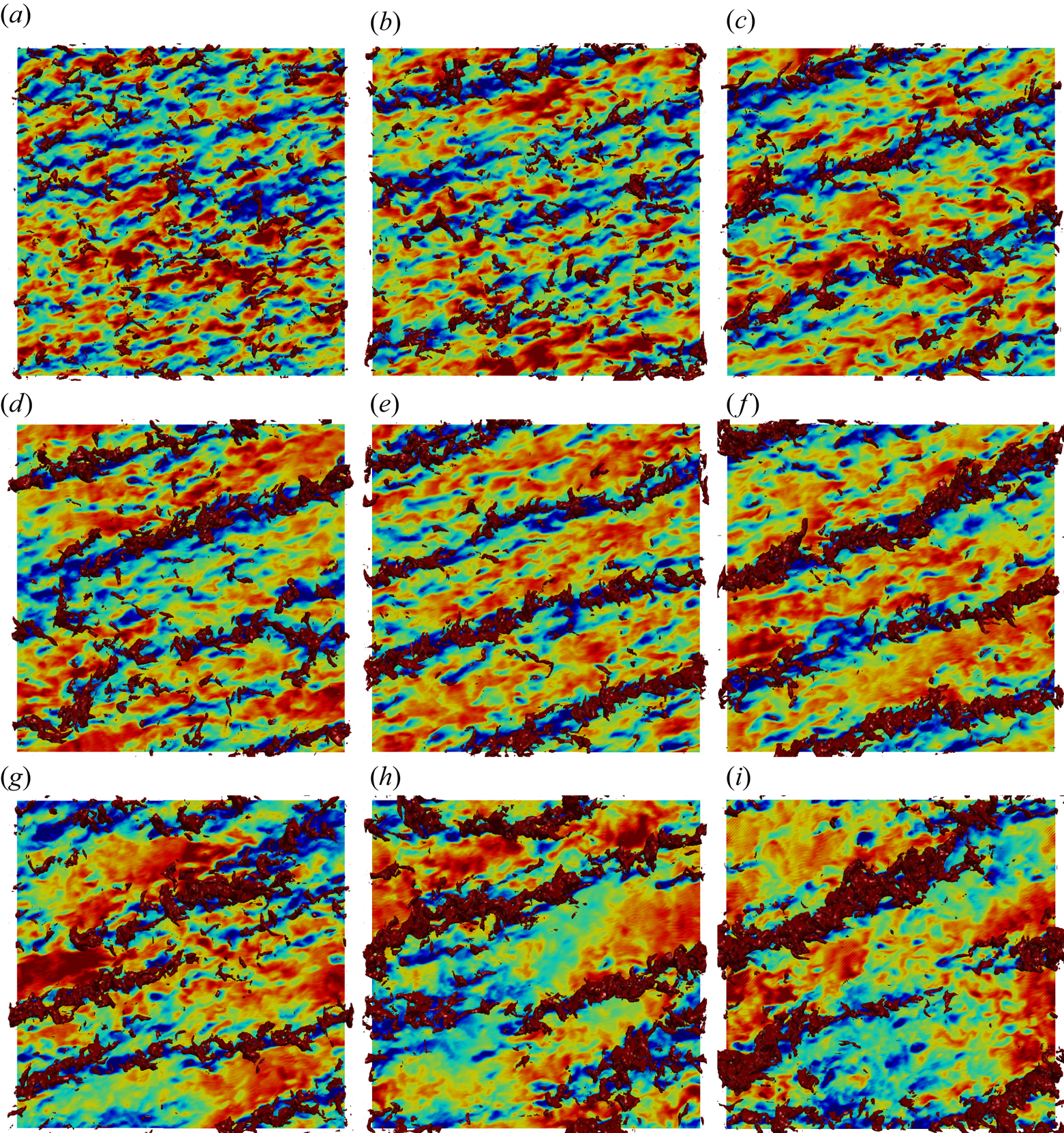
Figure 7. Simultaneous visualization of isocontours of  $x$-component velocity on the
  $z/z_i=0.1$ plane in unrotated coordinates (the underlying blue–green–red isocontours) and a single isosurface of vertical velocity (dark red) at a
  ${w^{\prime }}$ level of
  $2\sigma _w$ (
 $\sigma =$ standard deviation). The isocontours of
  $u^{\prime }$ vary from
  $-2\sigma _u$ (dark blue) to
  $+2\sigma _u$ (bright red); the solid green colour is close to zero. The dark blue and blue isocontours identify coherent ‘low-speed streaks’ generated by mean shear rate, which is dominant in the surface layer. The bright red/orange isocontours identify ‘high-speed streaks’. The dark red isosurface identifies concentrations of strong buoyancy-driven updraughts in the mixed layer. From these images, one can identify the spatial relationships between shear-driven low-speed streaks below and updraughts above, as a function of stability state. The transitional states discussed in the text are indicated with bold in the following: (a)
  $-z_i/L=0.000$; (b)
  $-z_i/L=0.304$; (c)
  $-z_i/L=\boldsymbol {0.433}$ (critical); (d)
  $-z_i/L=0.744$; (e)
  $-z_i/L=0.916$; (f)
  $-z_i/L=\boldsymbol {1.08}$ (maximally coherent roll state); (g)
  $-z_i/L=1.42$; (h)
  $-z_i/L=\boldsymbol {2.86}$ (transition to the canonical moderately convective ABL); and (i)
  $-z_i/L={3.84}$.
Figures 7(a) and 7(b) correspond to subcritical instability states. At these states, the regions of concentrated vertical velocity visually display much less coherence than do the low-speed streaks below, with relatively little apparent alignment between the updraughts and streaks. In contrast, the turbulence at critical and supercritical instability states (figures 7c and 7d) indicate higher levels of strength and organization in vertical velocity in the mixed layer. These developing vertical updraughts not only are more elongated in the horizontal, consistent with the dramatic increase in streamwise integral scales of horizontal and vertical velocity fluctuations (figure 3), but also are much more obviously aligned with the underlying low-speed streaks in the surface layer. Indeed, comparison of the supercritical state (figure 7d) with the subcritical state (figure 7b) clearly shows a strong change in both the structure of updraughts – they become more concentrated, well defined and coherent along the streaks – and more obvious alignment with the stronger low-speed streak structures below. Khanna & Brasseur (Reference Khanna and Brasseur1998) argued that an increased alignment between mixed layer updraughts above and surface layer streaks below results from the near-surface concentration of higher-temperature fluid within shear-generated, highly coherent, low-speed streaks, concentrating buoyancy force there and driving flow vertically within sheet-like regions of concentrated vertical velocity fluctuations. In this way, the low-speed streaks operate as ‘seeds’ to updraughts when buoyancy force drives vertical motions in the mixed layer post-critical.
In summary, we see from both observation (figure 7) and quantification (figure 3) that the streamwise coherence of surface layer elongated streaks suddenly increases with increasing surface heating (and  $-z_i/L$) at the critical state (
 $-z_i/L = 0.433$). In the post-critical states, observations up to
  $-z_i/L =1.08$ (figures 7d–7f) indicate that the low-speed streaks become increasingly well defined and coherent visually even as the streamwise coherence length
  $L_{11,1}$ decreases with increasing
  $-z_i/L$ (figure 3a).
5. Development of large-scale rolls at a maximum coherence stability state
In this section we analyse how increases in surface heat flux to the post-critical ABL states leads to a second ‘maximum coherence state’ associated with ‘large-scale rolls’.
5.1. The transition from critical to ‘maximum coherence’ stability states
We have learned that the transition between the neutral and moderately convective states in the equilibrium ABL is non-monotonic, with a critical stability state occurring at 1 %–2 % of peak midday flux and sudden changes in streak and updraught structure. Specifically, the streaks elongate in the horizontal and thicken in the vertical with increase in  $-z_i/L$ such that the aspect ratio
  $L_{11,1}/L_{11,3}$ in the upper surface layer changes from nearly
  $5$ in the neutral ABL to
  ${\sim }9$ in the critical ABL state (figures 3a, 5a and 6). The updraughts elongate, but do not thicken over this critical transition, with the aspect ratio
  $L_{33,1}/L_{33,3}$ increasing from
  ${\sim }1$ to
  ${\sim }5$ (figures 3b, 5b and 6) in the mid mixed layer, suggesting amalgamation into ribbon-like structures. The centre of these elongated updraughts lies just over that of the thickened streaks below (figure 5). Interestingly, the fact that the vertical extent of the updraughts has not changed significantly at the critical state suggests that the updraughts are not yet sensitive, in the vertical, to direct forcing from buoyancy. However, the concentrations of horizontal velocity fluctuations have thickened in the vertical to now partially overlap with updraughts (figure 5). We argue that this restructuring at the critical state with sudden spatial overlap between the upper margins of the streaks and lower margins of the updraughts yields a dynamically altered ABL in how it responds to further increases in surface heat flux post-critical as discussed below.
Continued increases in surface heating (and buoyancy force) post-critical appear to strengthen the coherence of the shear-driven horizontal fluctuations within low-speed streaks (figures 7d–7f) in spite of the decrease in  $L_{11,1}$ (figure 3a). The decrease in
  $L_{11,1}$ post-critical appears to be driven by increasingly incoherent concentrations of the high-speed horizontal velocity fluctuations in between increasingly coherent shear-driven low-speed streaks. The nonlinear interplay between surface-heating-induced buoyancy force and shear-driven streak coherence manifests differently in the dynamically altered supercritical ABL as compared to the subcritical ABL. Whereas horizontal coherence lengths of both horizontal and vertical fluctuations respond mildly to slight increases in surface heat flux subcritical, visualizations (figure 7) and quantifications (figure 5) show that further increases in
  $-z_i/L$ post-critical, lead to vertical extension of the ribbon-like concentrations of updraughts. This vertical extension is in response to increases in buoyancy force (figure 6), even as the updraughts continue to extend in the horizontal (figure 3b). This is particularly the case away from the surface where vertical velocity is not damped, suggesting that the critical state initiates a new susceptibility of updraughts to the influence of buoyancy.
The visualizations in figures 7(c)–7(f) indicate that the critical state initiates a strong spatial relationship between the horizontally extending and vertically growing updraughts above, and the fattened low-speed streaks below. The supercritical regime is characterized by spatial correlation between streaks and updraughts – turbulence structures created by fundamentally different physical mechanisms that strengthen with increasing surface heat flux and  $-z_i/L$. This leaves the supercritical states receptive to buoyancy and buoyancy-induced vertical motions that increasingly couple the lower and upper atmosphere with increasing
  $-z_i/L$. We argue that this post-critical regime with spatial correlation between streaks and updraughts (figure 7) is the initiation of the Khanna & Brasseur (Reference Khanna and Brasseur1998) mechanism, whereby low-speed streaks act as seeds for updraughts.
Figure 3 shows the existence of two well-defined peaks in horizontal coherence length:  $L_{11,1}$, which peaks at the critical state
  $-z_i/L=0.433$ and declines monotonically with
  $-z_i/L$ post-critical; and
  $L_{33,1}$, which peaks at
  $-z_i/L = 1.08$, a ‘maximum coherence state’ for updraughts. The horizontal scale of the updraughts increases by approximately
  $70\,\%$ in the mixed layer from the critical to maximum coherence states (figures 3b and 5b), an increase of approximately 8 times the scale at the initial neutral ABL state. The change in the relative streamwise coherence scale of updraughts to streaks,
  $L_{33,1}/L_{11,1}$, is shown in figure 8(a). Over the range of supercritical states
  $-z_i/L\sim 0.433\text {--}1.08$, where the horizontal scale of the updraughts peaks, the horizontal scale of the streaks (
 $L_{11,1}$) has decreased to become only
  ${\sim }30\,\%$ larger than that of the updraughts at the maximum coherence state. Figure 8(a) shows that the streamwise coherence length of updraughts (
 $L_{33,1}$) approaches that of the streaks (
 $L_{11,1}$) with increasing
  $-z_i/L$ post-critical, with a major reduction in the rate of increase in
  $L_{33,1}/L_{11,1}$ with
  $-z_i/L$ taking place as
  $-z_i/L$ increases from below to above the maximum coherence state,
  $-z_i/L=1.08$.
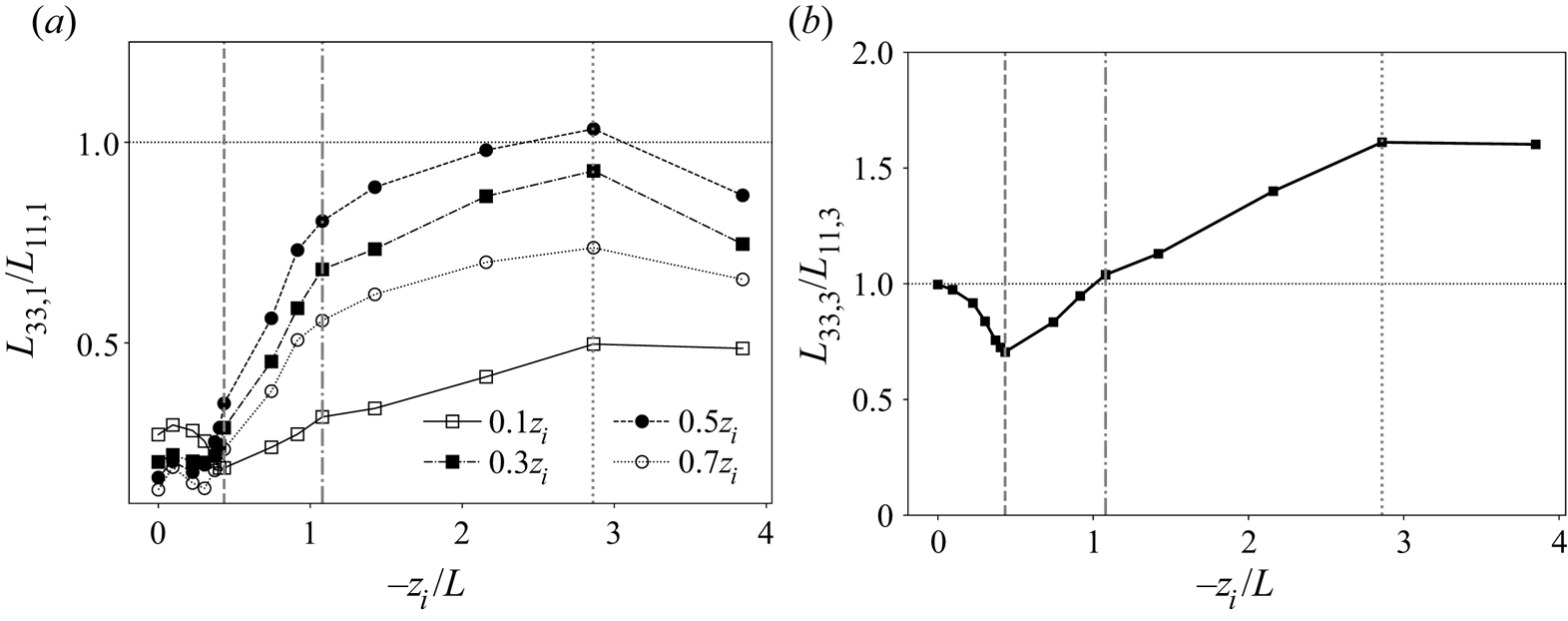
Figure 8. Transition in the ratio of coherence lengths of vertical to horizontal velocity fluctuations with stability state  $-z_i/L$ at fixed heights: (a) streamwise coherence lengths and (b) vertical coherence lengths referenced to
  $0.1z_i$. The three vertical lines in grey correspond to the key transition states:
  $-z_i/L=0.433$ (dashed),
  $-z_i/L=1.08$ (dot-dashed) and
  $-z_i/L=2.86$ (dotted). The horizontal dotted line at 1.0 identifies the transition states at which the scales of horizontal and vertical velocity fluctuations match.
The maximum coherence state is characterized not only by a peak in horizontal scale of the updraughts (figure 3b) and by a sudden change in the relative rates of increase in horizontal scale of updraughts versus streaks with  $-z_i/L$ (figure 8a), but also by the changes in the vertical scales of updraughts versus streaks. As shown in figure 6, increased buoyancy force extends the updraughts vertically (
 $L_{33,3}$) while the vertical thickness of the streaks (
 $L_{11,3}$) reduces. Other than the neutral state where vertical velocity fluctuations are driven indirectly by mean shear, there is one stability state where the vertical correlation length of buoyancy-induced updraughts matches the vertical scale of the shear-driven streaks: the maximum coherence state
  $-z_i/L=1.08$ (figure 6), with strong vertical overlap between them. However, as surface heat flux and
  $-z_i/L$ increase beyond the maximum coherence state, the thickness of streaks continues to decrease and that of the updraughts continues to increase, as shown in figure 8(b), where the ratio of vertical length scales,
  $L_{33,3}/L_{11,3}$, is plotted against
  $-z_i/L$. Similar to the ratio of horizontal scales shown in figure 8(a), the rate of increase in
  $L_{33,3}/L_{11,3}$ with
  $-z_i/L$ suddenly decreases at the maximum coherence state where the ratio passes through 1, and eventually saturates at
  $-z_i/L\sim 3$ (§ 6.2).
5.2. Large-scale rolls at the maximum coherence state
A key characteristic of the post-critical equilibrium ABL state is the progressive increase in the spatial overlap between streaks and updraughts (figure 7) with increases in instability. In this new supercritical ABL state the vertical motions not only are more receptive to buoyancy, but also thicken in the vertical to increasingly couple the lower and upper ABL with increases in surface heat flux. A manifestation of this coupling is ‘large-scale rolls’, a well-known structural feature of the ABL consisting of  $z_i$-scale rows of highly elongated updraughts between broader downdraught regions in the presence of mean streamwise flow, creating overall streamwise helical patterns that move warmer air to the capping inversion and cooler air to the ground. Large-scale rolls are often described in the literature in relationship to parallel lines of clouds near the capping inversion that are created by the condensation of moisture carried aloft within the coherent sheet-like updraughts (LeMone Reference LeMone1973; Etling & Brown Reference Etling and Brown1993; Weckwerth et al. Reference Weckwerth, Wilson, Wakimoto and Crook1997, Reference Weckwerth, Horst and Wilson1999).
One can study the changes in ABL streamwise coherence structure across the boundary layer (figure 5) as it transitions from the critical to the maximum coherence states to derive insights into the formation of rolls. The updraughts (figure 5b) transition from subcritical to critical (blue to red symbolled curves) by the sudden development of a strong well-defined peak in streamwise coherence length in the mid mixed layer ( $z/z_i\approx 0.44$). In the transition to maximum coherence state (from red to yellow symbolled curves) the peak broadens over the mixed layer as the updraughts amalgamate in the horizontal and thicken in the vertical. By contrast, after the horizontal scales of the horizontal fluctuations (
 $L_{11,1}$) increase at the critical state and peak in the lower mixed layer (
 $z/z_i\approx 0.34$), as shown by the red symbolled curve in figure 5(a), the transition to the maximum coherence state
  $-z_i/L=1.08$ involves a complete restructuring of streamwise coherence structure across the ABL. The transition is to one that, we argue, reflects the formation of maximally coherent large-scale rolls. In particular, the peak in
  $L_{11,1}$ in the critical state collapses to a local minimum while two new peaks in
  $L_{11,1}$ appear near the upper and lower ABL, where vertical motions are suppressed. A smaller peak (
 $L_{11,1}/z_i\approx 1.56$) appears in the upper surface layer (
 $z/z_i\approx 0.22$) while a larger peak (
 $L_{11,1}/z_i \approx 1.70$) appears just below the capping inversion (
 $z/z_i\approx 0.88$). The upper peak, we argue, arises from strong vertical velocities, induced in updraughts highly receptive to buoyancy, that are forced horizontal by blockage at the capping inversion. This reflects the maximum coherence state, where the streamwise coherence length of updraughts (
 $L_{33,1}$) is maximum in the mixed layer. In this way the large-scale roll state is distinguished by its cylindrical topology – exceptionally strong horizontal coherence of vertical velocity in the mixed layer combines with exceptionally strong horizontal coherence of horizontal velocity fluctuations (
 $L_{11,1}$) in the upper boundary layer. This change in morphology of ABL coherent structure initiates the existence of roll eddies and corresponds to the matching of vertical coherence length of updraughts with that of the streaks (figures 6 and 8b).
Figure 7 visually illustrates the transition to large-scale rolls in the approach to the maximum coherence state. At stability states below and above  $-z_i/L=1.08$, many small-scale concentrations of low-speed horizontal velocity fluctuation are observed between the dominant updraughts that are aligned with the dominant low-speed streaks. The maximum coherence state (figure 7f) is characterized by exceptionally coherent updraughts that spatially overlap exceptionally coherent and extended low-speed streaks, with few low-speed horizontal fluctuations in between. Fluid particles that originate at the lower margins of the exceptionally strong updraughts (red isosurfaces) move vertically, on average, as they move longitudinally with the mean flow. At the capping inversion the fluid particles are forced horizontally towards the centreline between neighbouring updraughts, generating a local maximum in
  $L_{11,1}$. Between the updraughts, fluid particles are forced downward within less coherent downdraughts, where they are again forced horizontal by surface blockage, creating another local peak in
  $L_{11,1}$ and completing the helical structure of the large-scale rolls.
Because the lateral separation distance between coherent thermal updraughts scale on  $z_i$, the helical streamline patterns are expected to extend over multiple
  $z_i$ in the streamwise direction. Interestingly, while the streamwise coherence lengths of the vertical and horizontal velocity fluctuations peak at
  $1z_{i}\text {--}2z_i$ in the maximum coherence state, the visual streamwise extent of the coherent large-scale roll structure, in both figure 7 and in meteorological images of cloud-topped large-scale rolls, extend well outside the simulation domain of
  $7z_{i}\text {--}8z_i$. Cloud visualizations (Weckwerth et al. Reference Weckwerth, Wilson, Wakimoto and Crook1997, Reference Weckwerth, Horst and Wilson1999) suggest that the coherent large-scale rolls often extend over tens of
  $z_i$. This is consistent with simulations performed over an extended domain as reported in appendix A.3, where the rolls appear to extend beyond
  $O(10z_i)$ at the maximum coherence state.
In summary, as heat flux and  $-z_i/L$ continue to increase post-critical (
 $-z_i/L\gtrsim 0.433$), the dynamically altered supercritical ABL, with updraughts becoming more receptive to buoyancy force, undergoes a dramatic, albeit monotonic, change in its coherence structure towards a ‘maximum coherence state’ at
  $-z_i/L=1.08$. This special state is characterized by maximally coherent large-scale rolls realized as
  $L_{33,1}$ approaches
  $L_{11,1}$ in the mixed layer and when
  $L_{33,3}$ approximately matches
  $L_{11,3}$ in response to a strong spatial overlap between the lower margins of the updraughts and upper margins of the streaks, creating exceptionally strong coupling across the depth of the ABL. Thus, the formation of rolls is a manifestation of the Khanna & Brasseur (Reference Khanna and Brasseur1998) mechanism at a state with maximal global response to buoyancy force in the mixed and upper layers of the ABL, localized to exceptionally coherent low-speed streaks in the upper surface layer.
6. The near-neutral and moderately convective ABL
Here we describe the ABL structure within the subcritical and post-maximum-coherence stability states to complete the description of ABL transition with increases in  $-z_i/L$.
6.1. The subcritical stability states ($0\leq -z_i/L< 0.371$)

The subcritical stability states may be traditionally described as ‘near neutral’ – an equilibrium ABL with finite but sufficiently small levels of surface heat flux such that the ABL has properties ‘close’ to the neutral state. In principle, near-neutral states are characterized by negligible role of buoyancy force, with temperature effectively a passive scalar. The transition to temperature as an active scalar initiates near the critical stability state in the range  $-z_i/L\sim 0.371\text {--}0.433$ (figure 5), with very low levels of surface heat flux that increasingly destroys the near-neutral character of the ABL.
From neutral through  $-z_i/L\lesssim 0.304$, however, our simulations produce an ABL that appears to be roughly neutral. Interestingly, however, the streamwise velocity fluctuations – but not the vertical velocity fluctuations – respond mildly to the extremely low subcritical levels of heat addition to the neutral ABL. Figure 4(a) indicates small changes in the variance of streamwise velocity. Figures 3(a), 5(a) and 6 show small changes in both the streamwise and vertical coherence structure of the streamwise velocity fluctuations across the boundary layer, while figures 3(b), 5(b) and 6 indicate negligible subcritical response in the vertical velocity fluctuations. These results suggest the existence of mild, but measurable, impacts of extremely low-level surface heating on the streamwise velocity fluctuations – just below a critical level of surface heat flux that causes complete restructuring of ABL turbulence and a fundamental change from passive to active temperature response. It is interesting that this low-level response is entirely in the streamwise velocity fluctuations; vertical fluctuations respond only at and post-critical.
6.2. Transition to the ‘moderately convective’ stability state
The ‘maximum coherence state’ associated with highly coherent large-scale rolls (see § 5) is quantitatively characterized by a peak in streamwise coherence length of the amalgamated updraughts at  $-z_i/L = 1.08$ and preceded by a sudden change in ABL receptivity to surface heating at the critical state. Both of these transitions in ABL character are visually identifiable by the structure of horizontal versus vertical fluctuating velocity concentrations and the spatial relationships between them.
However, there is a third transition in ABL turbulence structure around  $-z_i/L = 2.86$ that is characterized quantitatively by asymptotes and peaks in scale relationships (figures 6 and 8) and qualitatively by changes in updraughts versus streak structure (figure 7). This occurs as increases in
  $-z_i/L$ move the ABL into the ‘moderately convective’ states described in previous studies (Moeng & Sullivan Reference Moeng and Sullivan1994; Khanna & Brasseur Reference Khanna and Brasseur1998). Figure 6 shows that the vertical coherence lengths of both vertical and horizontal fluctuating velocities asymptote at
  $-z_i/L > 2.86$, suggesting a regime whereby additional increases in surface heat flux do not cause much change in their vertical scales. Post-critical, the vertical scale of updraughts monotonically increases while that of the streaks decreases monotonically (figure 6). The ratio
  $L_{33,3}/L_{11,3}$ passes through 1 at the maximum coherence state and continues to grow to a plateau at
  $-z_i/L > 2.86$ (figure 8b), where the vertical scale of updraughts is approximately
  $56\,\%$ greater than that of streaks.
The horizontal coherence lengths of the updraughts versus streaks, by contrast, approach one another with the ratio of horizontal scales  $L_{33,1}/L_{11,1}$ (figure 8a) hovering near 1 in the mixed layer at
  $-z_i/L\gtrsim 2.86$. Near the ground, where vertical motions are suppressed (
 $z/z_i=0.1$), the horizontal scales of both vertical and horizontal fluctuations reduce slowly when
  $-z_i/L$ exceeds 2.86 (figure 3) so that the ratio
  $L_{33,1}/L_{11,1}$ plateaus with streaks nearly twice as long in the horizontal as updraughts, in contrast to the mixed layer.
Visualizations in figures 7(f)–7(i) clearly show that the horizontal coherence of streaks and updraughts breaks down at higher  $-z_i/L$ beyond the maximum coherence state. In addition, the spatial correlation between streaks and updraughts, which starts at the critical state
  $-z_i/L=0.433$ and strengthens up to maximal spatial correlation at
  $-z_i/L=1.08$, reduces in the transition from the maximum coherence state to the moderately convective limit. Presumably, this process will continue into the fully convective state as the impacts of buoyancy on vertical motions fully dominate impacts of shear and the rolls transition to turbulent Rayleigh–Bénard convection cells. What distinguishes the moderately convective ABL is the continued importance of shear rate and, correspondingly, a roll-like structure, even as convection increasingly dominates and roll coherence diminishes.
Analysis of the ABL streamwise coherence structure (figure 5) shows that the horizontal scales of both vertical and horizontal velocity fluctuations reduce monotonically at all heights as the stability state transitions from  $-z_i/L=1.08$ (yellow curves) to
  $-z_i/L=3.84$ (green curves). However, in comparing the moderately convective states (green curves) with the neutral state (blue curves), the streamwise coherence lengths of horizontal velocity fluctuations in the moderately convective state are below that of the streaks in the neutral state. By contrast, the horizontal scale of the vertical fluctuations remains well above that in the neutral state, by a factor of 3 in the mixed layer. This difference between the neutral and moderately convective states reflects the two different sources of vertical velocity fluctuation, namely from buoyancy (post-critical) and indirectly from shear (in the neutral). Correspondingly, in the transition to moderately convective ABL, the buoyancy-driven mixed layer velocity scale
  $w^{*}$ progressively dominates the shear-driven surface layer velocity scale
  $u^{*}$ (figure 2b).
7. Summary and conclusions
It is surprising that the coherence length of the streaks should dramatically increase with the addition of minuscule levels of heat flux through the ground into a previously neutral ABL. Given that both streamwise turbulent velocity fluctuations and highly coherent low-speed streaks are produced by the impact of mean shear rate on underlying turbulence fluctuations (Rogers & Moin Reference Rogers and Moin1987; Lee et al. Reference Lee, Kim and Moin1990), one would expect that the addition of buoyancy force would interfere with and reduce coherence generated by shear–turbulence interactions. We learn that this interference initiates only after ABL turbulence has first responded to slight surface heating by suddenly changing its structure. At the critical state  $-z_i/L \approx 0.43$, streamwise streaks have extended horizontally, thickened vertically and increased in aspect ratio, while concentrations of vertical velocity amalgamate and extend in the streamwise direction. These vertical velocity concentrations change from relatively incoherent, aspect ratio order
  $1$, structures into ribbon-like updraughts with aspect ratio
  ${\sim }5$. Furthermore, as the updraught ribbons form at the critical state in the mixed layer, they increase in alignment with low-speed streaks in the surface layer. Because the streaks have fattened vertically, the upper half of the streaks now overlap with the lower half of the ribbon updraughts, enhancing communication between streaks and thermals.
Indeed, we argue that the sudden transition in ABL turbulence structure at the critical stability state initiates a new receptivity to buoyancy force together with a new spatial relationship within the changed ABL, both of which strengthen with increased surface heat flux. This new receptivity causes the ribbon-like updraughts created at the critical state to respond to additional surface heating by extending vertically while the streaks reduce in thickness from a peak at the critical state. More importantly, the mixed layer updraughts continue to extend horizontally in response to additional heating as they become more aligned with low-speed streaks below, maintaining aspect ratio  ${\sim }5$. Visually, this process occurs coincident with increased streamwise extension of highly coherent low-speed streaks, even as the coherence length of horizontal velocity fluctuations reduces, implying major loss of streamwise coherence in the high-speed regions. We argue that the increased alignment of thermal updraughts above with coherent low-speed streaks below as heat flux increases from critical is a manifestation of the Khanna & Brasseur (Reference Khanna and Brasseur1998) mechanism whereby the low-speed streaks are described as sources of buoyancy force and thermal generation.
As surface heat flux increases above critical, the streamwise coherence length of the ribbon-like thermals increases to a peak at  $-z_i/L\approx 1$ as the thermals continue to extend vertically. We argue that this peak in streamwise coherence length of the mixed layer updraughts, coincident with exceptionally strong alignment with coherent low-speed streaks in the surface layer below, is associated with maximally coherent ‘large-scale rolls’ – helical structures that fill the ABL and globally connect the lower and upper boundary layer regions. Field observations indicate that large-scale rolls can extend downstream for tens of capping inversion heights. Our analysis suggests that the transition to the roll state requires first a restructuring of the neutral ABL to a critical state that differs substantially in turbulence structure from the neutral ABL. Whereas the relatively small and incoherent updraught regions in the neutral state are not receptive in the vertical to increases in surface heating, the updraughts in and above the critical state are. This new receptivity allows the critical state thermals, greatly extended in the horizontal but not in the vertical, to now extend vertically with increased surface heat flux and create the strong thermal updraughts within the maximally coherent large-scale rolls at
  $-z_i/L\sim 1$.
Interestingly, the maximally coherent roll state is defined quantitatively by maximum coherence in streamwise, rather than vertical, coherence length of vertical velocity with increasing  $-z_i/L$. As surface heat flux and
  $-z_i/L$ increase above the maximum coherence state, the thermals continue to grow in the vertical to a maximum at
  $-z_i/L\sim 3$. Horizontal coherence, however, decreases and, visually, the structure of the large-scale rolls progressively deteriorates. As the vertical coherence length of the thermal updraughts asymptotes to a maximum at
  $-z_i/L\sim 3$, the streamwise scales of both vertical and horizontal velocity fluctuations decrease and assume nearly equal magnitudes in the mixed layer at
  $-z_i/L\sim 3$. The asymptotic limit
  $-z_i/L\sim 3$, we argue, represents the transition from the ‘roll’ state to the canonical ‘moderately convective’ ABL.
It should be noted that, because maximally coherent large-scale atmospheric rolls have been observed indirectly through cloud visualization to extend tens of kilometres in the horizontal (see §§ 1 and 5.2), it is likely that our horizontal domain of 5 km does not fully capture horizontal correlations at the maximum coherence state. Appendix A.3 describes a study in which the horizontal domain was doubled in the  $x$ and
  $y$ directions. We observe the impact on horizontal integral scales at the critical and maximum coherence states,
  $-z_i/L = 0.43$ and
  $1.08$, as well as at the roll stability states at
  $-z_i/L > 1.08$. However, the key results presented in this study remain unchanged. In fact, the larger domain accentuates behaviour at the critical stability state. Underlying this result, we find that the streamwise two-point correlations ((2.9)) are generally close to zero at the end of the integration domain with the exception of the critical and maximum coherence states
  $-z_i/L = 0.43$ and
  $1.08$. For these two special states, the streamwise correlation coefficient of streamwise velocity fluctuations at the end of the correlation domain is
  $\sim 0.35$ at the critical state and
  ${\sim }0.2$ at the maximum coherence state in the mixed layer. Interestingly, however, these numbers do not change much when the horizontal domain is doubled, implying that much larger domains would be required in the horizontal to fully capture all horizontal integral scales. However, it also indicates that the horizontal integral scales are underestimated at the critical and maximally coherent roll states in the current study and that the critical state is, in reality, stronger.
The mechanisms that underlie the restructuring of the ABL at the very low levels of surface heat flux in the critical state  $-z_i/L\approx 0.43$ are unknown. Interestingly, we find that, whereas the streamwise coherence structure of vertical velocity fluctuations is suddenly changed at the critical state, subcritical levels of surface heat flux only significantly impact horizontal velocity fluctuations, and primarily in the thickening of the streaks in the vertical. It is surprising that, even as buoyancy force increases with increasing surface heat flux subcritical, there is no significant increase in vertical velocity variance. Even more surprising is that increasing surface heat flux subcritical changes the vertical coherence of horizontal velocity fluctuations but not the vertical coherence of vertical velocity fluctuations.
An important result from the current study is that it is highly unlikely that an ABL in equilibrium can exist in the neutral state over land, particularly between sunrise and sunset. The extremely low global stability parameter at the critical state corresponds to surface heat flux so low to make it highly likely that a turbulent post-critical ABL is generated almost immediately after sunrise with turbulence structure very different from neutral, particularly in the structure of the updraughts. Whereas the nocturnal ABL is generally stable, the passage of  $z_i/L$ through 0 in the transition between day and night is associated with highly non-stationary and non-equilibrium dynamics outside the canonical description of the neutral ABL.
Theory and experiment are needed, from which an understanding of the mechanisms underlying the unexpected dynamics uncovered in the current study can be gained. The fact that the maximum coherence state is characterized by horizontal, rather than vertical, coherence of thermal updraughts indicates a complex dynamical interplay between shear-modulated turbulence near the ground and buoyancy-modulated turbulence away from the ground, with sources near the ground that are directly impacted by mean shear. Whereas the current study uncovers much previously unknown ABL dynamics, it also uncovers many intriguing questions that beg an explanation.
Funding
The research has been supported by the Department of Energy EERE Office under grant DE-EE0005481. Additionally, B.J. was supported by NASA OK-EPSCoR seed grant. Computer resources were provided by the Oklahoma State University HPCC, National Science Foundation XSEDE award TG-ATM0007.
Declaration of interests
The authors report no conflict of interest.
Appendix A. The overshoot and simulation design impacts
A.1. Removal of the overshoot using the methodology of BW10
Grid design for accurate LES prediction of the ABL was discussed in Brasseur & Wei (Reference Brasseur and Wei2010, BW10) in the context of the development of a methodology to remove the well-known overprediction of mean shear rate in the surface layer (‘the overshoot’) of the neutral ABL. Although this analysis was developed for the neutral case, we applied the methodology in the current study in all simulations and were pleased to find that the method was successful in minimizing the overshoot also for the convective cases. BW10 showed that suppression of the overshoot was part of a process required to design LES both to satisfy the LOTW and to produce grid independence. In this section we summarize the methodology and show the suppression of the overshoot in our LES study. In the subsequent sections we briefly present a grid refinement study and discuss the influence of the domain size.
The BW10 approach is based on a theory that relates three non-dimensional LES parameters,  $\mathfrak {R}$,
  ${Re}_{LES}$ and
  $N_{\delta }$, through the following model-independent expression:
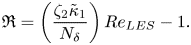 \begin{equation} \mathfrak{R}=\left( \frac{\zeta_2\tilde{\kappa}_1}{N_{\delta}} \right) {Re}_{LES}-1. \end{equation}
Here  $\mathfrak {R}=[ T_R/T_S ]_1$ is the ratio of resolved to SFS mean turbulent shear stress at the first grid level;
  ${Re}_{LES}=u^{*}z_i/\nu _{LES}$ is the ‘LES Reynolds number’ based on an ‘LES viscosity’
  $\nu _{LES} \equiv [ T_S/( 2\rho \langle s^{r}_{13} \rangle ) ]_1$, where
  $s^{r}_{13}$ is the resolved shear strain rate;
  $N_{\delta }$ is the number of uniformly spaced grid points in the boundary layer in the vertical;
  $\zeta _2$ is an order
  $1$ constant; and
  $\tilde {\kappa }_1$ is of the order of the von Kármán constant (it is the von Kármán constant when the LOTW is correctly predicted). For eddy viscosity representations of the SFS stress tensor, BW10 show that
 \begin{equation} \mathfrak{R}\sim 1/D_t \quad \text{and}\quad {Re}_{LES} \sim N_{\delta}/D_t,\quad\text{with } D_t=C^{a}_t A^{b}_R, \end{equation}
where  $A_R=\varDelta _x/\varDelta _z=\varDelta _y/\varDelta _z$ is the aspect ratio of the grid cells and
  $C_t$ is the model constant. The values of
  $a$ and
  $b$ depend on the specific eddy viscosity closure: for the one-equation model
  $a=1$ and
  $b=8/9$ with
  $C_t \equiv C_k$ ((2.4)), and for the Smagorinsky closure
  $a=1$ and
  $b=4/3$ with
  $C_t=C^{2}_s$ (
 $C_s$ being the Smagorinsky constant).
Equation (A1) contains a mix of predicted physical quantities and two grid-related quantities: the resolution of the grid in the vertical ( $N_{\delta }$) and the aspect ratio
  $A_R$ of the effective grid cells (i.e. after dealiasing). Together with the model constant,
  $\mathfrak {R}$ characterizes the impact of modelled friction on LOTW scaling. The effective Reynolds number for the LES is shown to depend on both effective friction at the resolved scales and vertical grid resolution. BW10 showed that, to remove the overshoot,
  $\mathfrak {R}, {Re}_{LES}$ and
  $N_{\delta }$ should exceed, but remain close to, the critical values
  $\mathfrak {R}^{*}\sim O(1)$,
  ${Re}^{*}_{LES}$ and
  $N^{*}_{\delta }$, which depend on the closure. (If the method applies also to the non-neutral ABL, the critical values probably also depend on
  $-z_i/L$.) For the neutral ABL calculated with the Smagorinsky model, BW10 empirically estimated
  $\mathfrak {R}^{*}\sim 0.85$,
  ${Re}^{*}_{LES}\sim 350$ and
  $N^{*}_{\delta }\sim 40\text {--}45$. Because the current simulations apply a one-equation eddy viscosity model and include convective states, the critical values are likely to be significantly different from the BW10 estimates for the neutral ABL. Nevertheless, we indicate the BW10 estimates in figure 9 for comparison, where each simulation evaluated in the current study is shown on a plot of
  $\mathfrak {R}$ against
  ${Re}_{LES}$. This visual representation of (A1), called ‘the
  $\mathfrak {R}$–
 ${Re}_{LES}$ parameter space’, is a useful tool to systematically adjust the LES design to remove the overshoot. This is because, although the critical values
  $\mathfrak {R}^{*}\sim O(1)$,
  ${Re}^{*}_{LES}$ and
  $N^{*}_{\delta }$ may not be known precisely, they are known roughly and the trends are well displayed. The aim is to place the LES roughly in the corner of the greyed-in region in figure 9, where the three parameters just exceed their critical values (BW10 called this region the ‘high-accuracy zone’, or HAZ).
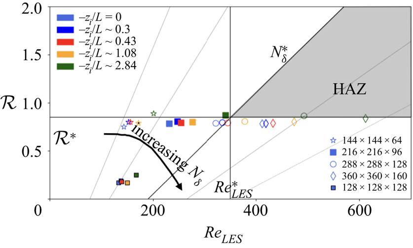
Figure 9. The  $\mathfrak {R}$–
 ${Re}_{LES}$ parameter space with the parameters for the LES analysed in the current study shown. The solid symbols are for the simulations used in the main body of the paper, where the small solid symbols are for the initial LES displaying clear overshoots (
 $128\times 128\times 128$) and the larger solid symbols are the simulations adjusted to remove the overshoot and analysed in the study (
 $216\times 216\times 96$). The open symbols are additional simulations used in the grid convergence study discussed in appendix A.2. The solid lines for
  $\mathfrak {R}^{*},{Re}^{*}_{LES}$ and
  $N^{*}_{\delta }$ are drawn at the nominal values from BW10 for LES of the neutral ABL using the Smagorinsky SFS stress model.
BW10 found that, whereas all three critical values must be surpassed to satisfy the LOTW and achieve grid independence, the removal of the overshoot was particularly sensitive to the requirement  $\mathfrak {R} > \mathfrak {R}^{*} \approx 1$. In figure 10 we plot with solid lines the LES before versus after we successfully removed the overshoot (after multiple systematic experiments using the
  $\mathfrak {R}$–
 ${Re}_{LES}$ parameter space). The initial
  $128\times 128\times 128$ effective grid, shown on figure 10 with solid grey lines, produces a clear overshoot consistent with the location of the simulation on the
  $\mathfrak {R}$–
 ${Re}_{LES}$ parameter space (figure 9). The simulations analysed in the current study apply the
  $216\times 216\times 96$ effective grid shown with the thick solid lines in figure 10 with the overshoot removed. As discussed in BW10, the increase in
  $\varPhi _M$ at the first grid level is not associated with the overshoot, while the shift in the mean shear profiles towards the surface is a result of increased resolution in the vertical. The change in the grid is associated with a reduction in cell aspect ratio
  ${A}_{{R}}$ from 2.5 to 1.1. As per (A2a,b),
  $D_t$ reduced in magnitude before to after the overshoot was removed, causing
  $\mathfrak {R}$ to increase as shown in figure 9. The
  ${Re}_{LES}$ value is dependent on vertical grid resolution in addition to grid aspect ratio, leading to a change in
  ${Re}_{LES}$ from roughly 134 with the
  $128\times 128\times 128$ grid to 230 with the
  $216\times 216\times 96$ effective grid, a value significantly lower than the estimated critical value in BW10. Visually, figure 9 shows that the original LES was far from the HAZ and that the change in the cell aspect ratio moved the location of the simulation from a part of the
  $\mathfrak {R}$–
 ${Re}_{LES}$ parameter space that characterize strong overshoot to much closer to the HAZ. Correspondingly, the geometric grid increased from
  $\approx 4.7\ \textrm {million}$ to
  $\approx 10\ \textrm {million}$ cells.
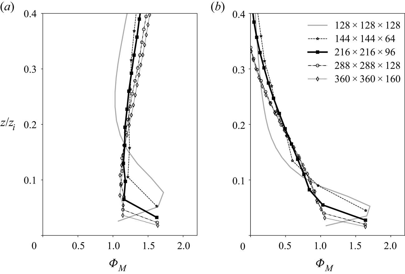
Figure 10. Mean shear normalized with inertial LOTW length and velocity scales,  $\varPhi _M(z)=({\kappa z}/{u^{*}})({\partial U}/{\partial z})$, plotted through the boundary layer: (a) the neutral ABL,
  $-z_i/L = 0$; and (b) the ‘maximum coherence state’ (see § 5),
  $-z_i/L = 1.08$. The solid grey lines without symbols show the initial LES developed on a
  $128\times 128 \times 128$ effective grid. The thick solid lines with symbols show the LES used in the current study developed on a
  $216\times 216\times 96$ effective grid. Also shown are the other resolutions used in the analysis of resolution impacts discussed in appendix A.2.
A.2. Analysis of grid resolution impacts
The grid design study using the methodology summarized in appendix A.1 makes clear that, for the rough-surface ABL applying a standard surface stress model (§ 2), a grid convergence study is sensible only with simulations that capture the LOTW. Furthermore, systematic changes in grid resolution must occur at the same effective grid cell aspect ratio so as to maintain  $\mathfrak {R}$ near critical ((A2a,b)). To this end, we carried out a series of simulations with the same grid aspect ratio as that of the
  $216\times 216\times 96$ effective grid used in this study (
 $A_R \approx 1.1$). The normalized mean shear profiles with one lower- and two higher-resolution grids are shown with open symbols in figure 10 for simulations of the neutral (
 $-z_i/L = 0$) and maximum coherent state (
 $-z_i/L = 1.08$) boundary layers. Although the comparison indicates small deviations at the two higher grid resolutions, the mean velocity is nearly grid-independent and very different from the
  $128\times 128\times 128$ effective grid case, which displays a clear overshoot. It is necessary that
  $N_{\delta }$ increase with increasing grid resolution at fixed grid cell aspect ratio. Therefore, as indicated by (A2a,b), whereas
  $\mathfrak {R}$ is constant,
  ${Re}_{LES}$ increases with increasing resolution. These characteristics are apparent in figure 9 where the systematically varying grid resolution results are shown for all stability states using open symbols. The observation that
  $\mathfrak {R}$ is nearly independent of grid resolution at fixed aspect ratio (and fixed
  $C_k$) for all stability states is consistent with the observation that the BW10 approach to remove the overshoot appears to apply also to convective states.
To demonstrate that the results presented in the current study using the  $216\times 216\times 96$ effective grid are mostly insensitive to increases in resolution when the overshoot is removed, we plot in figure 11 the two key integral scales,
  $L_{11,1}$ and
  $L_{33,1}$, against
  $-z_i/L$ using the two higher-resolution simulations at the same aspect ratio. The peaks both in
  $L_{11,1}$ at the critical state and in
  $L_{33,1}$ at the maximum coherence state are unchanged. Furthermore, the magnitudes of
  $L_{11,1}$ and
  $L_{33,1}$ as a function of
  $-z_i/L$ are nearly independent of grid resolution, with the exception of
  $L_{33,1}$ in the mixed layer, where the magnitude is higher at higher resolutions. Nevertheless, it is clear that the characteristics leading from the critical to maximum coherent states described in §§ 4 and 5 using data from the
  $216\times 216\times 96$ effective grid remain unchanged at higher resolution with fixed
  $A_R$.
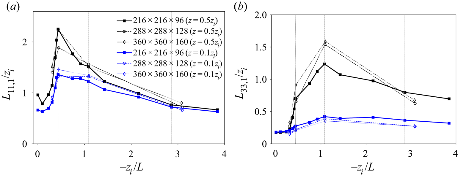
Figure 11. Comparison of normalized integral length scales at different grid resolutions: (a)  $L_{11,1}$ and (b)
  $L_{33,1}$ plotted against the stability state parameter,
  $-z_i/L$, near the surface (
 $z/z_i = 0.1$, blue) and in the mixed layer (
 $z/z_i = 0.5$, black). The simulations analysed in the current study (
 $216\times 216\times 96$) are shown using thick solid lines, while the higher-resolution cases (
 $233\times 288 \times 128$ and
  $360 \times 360 \times 160$) are shown using dashed and dotted lines.
In closing this section, we note that we previously obtained results similar to those in the current paper with a series of simulations that contained the overshoot (Jayaraman & Brasseur Reference Jayaraman and Brasseur2014, Reference Jayaraman and Brasseur2018); however, the characteristics at the critical states were less pronounced than in the current study. This suggests that the frictional content from the SFS stress model weakens the critical response described in the current study.
A.3. Analysis of domain size impacts
To study potential impacts of domain size on the key results and conclusions presented in the current study, we carried out new simulations with the same grid resolution (and cell aspect ratio) as used in the current analysis but at twice the horizontal domain width (10 km versus 5 km), as shown in figure 12. Of particular interest is the impact of domain width on the existence of the critical state at  $-z_i/L = 0.43$ and the maximum coherence stability state,
  $-z_i/L=1.08$, where
  $L_{11,1}$ is most highly extended at the critical state and
  $L_{33,1}$ at the maximum coherence state. Figure 12 shows that the existence of these special states clearly continues with the larger horizontal domain width. Indeed, the critical state (
 $-z_i/L = 0.43$) is more pronounced with the 10 km domain in the mixed layer, indicating some level of suppression of the horizontal extension of coherent structures by the use of a 5 km domain in the current study. Horizontal extension of vertical velocity coherence (
 $L_{33,1}$) is much less affected by the increase in horizontal domain width up to the maximum coherence state,
  $-z_i/L=1.08$. At
  $-z_i/L>1.08$, figure 12(b) shows that the 5 km horizontal domain constrains
  $L_{33,1}$, producing smaller horizontal integral scale magnitudes and more rapid reduction in streamwise correlation in the mixed layer compared to the 10 km domain. Furthermore, the slower breakdown of large-scale rolls for the 10 km domain with increasing
  $-z_i/L$ suggests that the ‘moderately convective’ state is approached at higher
  $-z_i/L$, possibly
  $\gtrsim 4$. In § 7, we discuss the analysis of two-point correlations in the context of the doubling the horizontal domain (not shown). This analysis confirms the impact of horizontal domain size on horizontal correlations at the maximum coherence state, accentuating the maximum coherence state but perhaps spreading it out over a range of
  $-z_i/L > 1.08$.
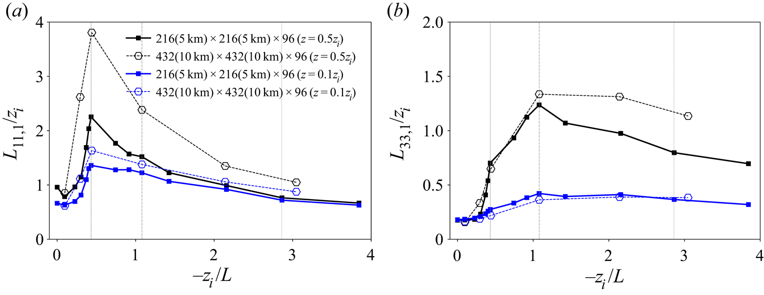
Figure 12. Comparison of normalized integral length scales from LES developed using double the horizontal domain width (10 km) as analysed in the current LES study with domain width of 5 km: (a)  $L_{11,1}$ and (b)
  $L_{33,1}$ plotted against the stability state parameter,
  $-z_i/L$, near the surface (
 $z/z_i = 0.1$, blue) and in the mixed layer (
 $z/z_i = 0.5$, black). The estimates from the smaller LES domain analysed in the current study (5 km domain width) are shown by the thick solid lines, while the simulations with double domain width (10 km) are shown by dashed and dotted lines.


 Open access