1. INTRODUCTION
Vehicle underwater passive navigation is an area of research with broad commercial and military application. Recently, there has been greater interest in using geophysical maps (for example gravity) for underwater navigation. A main aspect of underwater passive navigation is how to identify the vehicle location on an existing gravity map, and several matching algorithms as the Sandia inertial terrain aided navigation (SITAN) (Wang and Bian, Reference Wang and Bian2008; Liu et al., Reference Liu, Li., Zhang and Hou2011; Hostetler et al., Reference Hostetler and Andreas1983) and the Iterative Closest Contour Point (ICCP) (Cheng et al., Reference Cheng, Xiu and Luo2009; Garner, Reference Garner2002; Zhao et al., Reference Zhao, Wang and Wang2009) are the most prevalent methods that many scholars are using.
The SITAN algorithm uses a bank of Kalman filters to search the matching position based on recursive information from these Kalman filters. So SITAN is a real-time matching algorithm, but it also wastes a lot of time in the searching procedure and sometimes it misses position fixes because of the large quantity of searching points. This algorithm requires accurate initial position information and a linear change of gravity field, and it is mainly applicable for the carrier with a fixed trace. ICCP algorithms can give a matching path to correct the indicated path of an Inertial Navigation System (INS) only after getting enough samples, which makes its real-time quality not very good, and it is the most commonly used method in underwater gravity-aided INS.
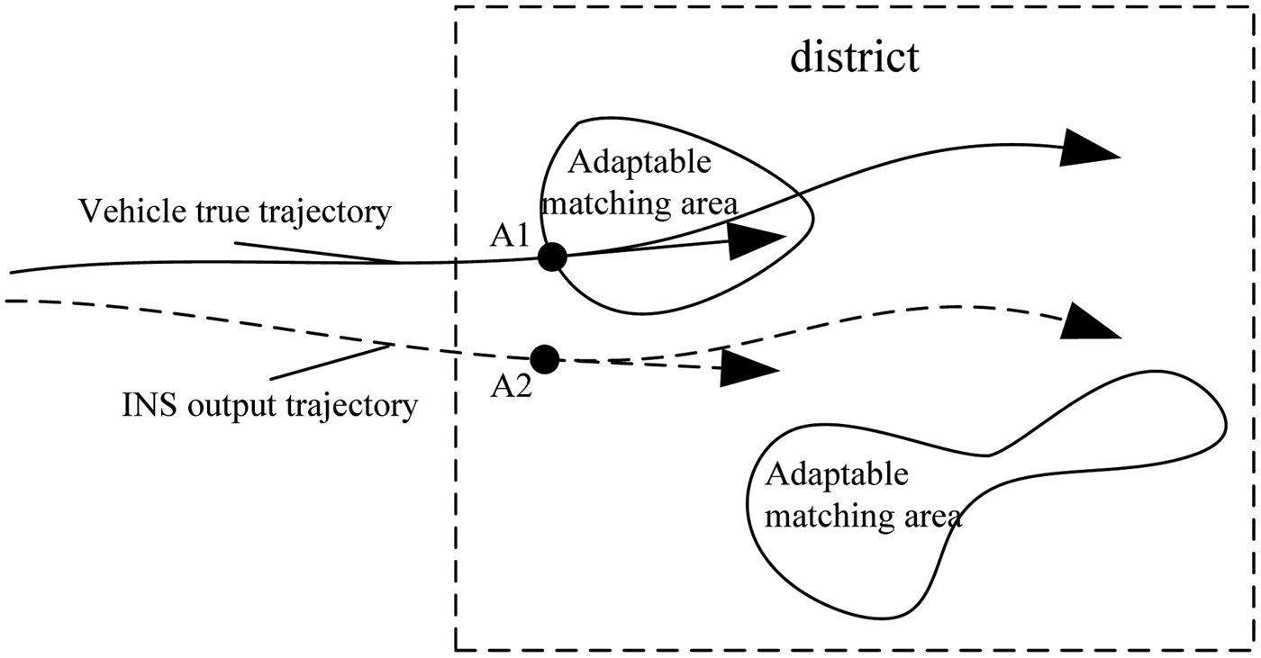
The ICCP algorithm is derived from static image matching in image recognition. For a gravity-aided inertial navigation system, the gravity reference map is only a one-dimensional “line graph” represented by “isograms”, rather than a two-dimensional graph acquired in the form of “video recording”. Such a line graph carries less available information for matching than the two-dimensional graph. Moreover, in order to improve resolution of the gravity reference map, the final “line graph” of the map is obtained by interpolation, which will inevitably result in errors for the map. The positioning accuracy of the gravity-aided inertial navigation system is related not only to the matching algorithm but also to the selection of gravity map matching area. The adaptable matching area is often chosen according to the average of standard deviation, local energy and roughness of gravity gradient (Cheng et al., Reference Cheng, Zhang and Cai2007. As shown in Figure 1, the suitable matching area of the gravity map is discontinuous due to its discrete distribution, so that a cumulative error occurs in the carrier position and navigation information exported by the INS in real time when the carrier enters into the applicable gravity matching area (Point A2 in Figure 1). These factors result in an essential difference in the gravity map matching criterion and optimum searching method. So there is an urgent need to discuss a new matching method.

Figure 1. Schematic diagram for initial gravity map matching error.
The possibility of triangle matching was first proposed by Golomb et al. (Reference Golomb, Streit and Robbins1978). Due to geometric features such as translation, rotation and stretch invariance of the matching triangle, the matching method based on the triangle constraint model has been widely used in the field of image matching in recent years (Guo and Cao, Reference Guo and Cao2012). Zhu et al. (Reference Zhu, Wu and Tian2007) proposed an image matching method based on a dynamic triangle constraint. Liu and An (Reference Liu and An2010) compared two similar triangles using the invariants of relative moment reflection to overcome the reflection transformation among matching images. Chen et al. (Reference Chen, Tian and Yang2006) proposed the fuzzy similarity of triangle matching by forming a triangle fuzzy function set with feature points. Qian and Wang (Reference Qian and Wang2008) gave a fuzzy expression of the triangle. Zheng et al. (Reference Zheng, Gao and Zhang2009) completed the vector triangle matching. The experiment results and application effects show that compared to the previous ICCP matching method, the matching method based on triangle constraint features better accuracy and stability. In addition, the triangle matching technique was introduced by Yang et al. (Reference Yang, Zhu and Zhao2014) to the gravity map-matching algorithm for the first time. They built a high-accuracy triangular observed quantity with a short time and high-accuracy measurement of the inertial navigation system.
From the SITAN and ICCP algorithms, it is known that the accurate initial position information is critical in the gravity map-matching algorithm. In this paper, the research will focus on the initial matching technique for a gravity map based on the triangle constraint model.
2. BASIC PRINCIPLE OF GRAVITY MAP MATCHING ALGORITHM BASED ON TRIANGLE CONSTRAINT MODEL
2.1. Matching Possibility of a Triangle
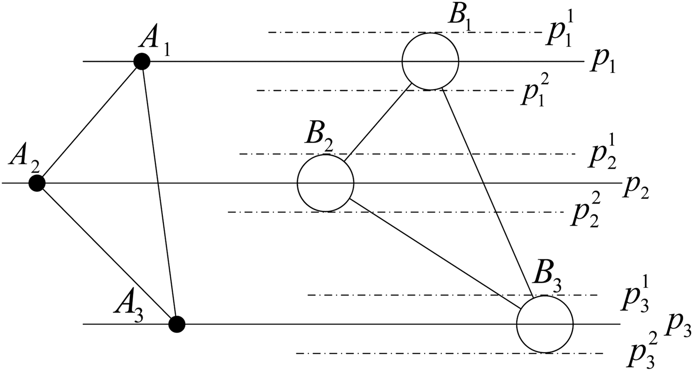
The matching possibility of a triangle is defined as follows: for two triangles ΔA1A2A3 and ΔB1B2B3 in the space R3, if there are three parallel lines p 1, p 2 and p 3 and rigid transformations σ and τ to enable σ (A i) and τ(Bi) to be on p i (i = 1,2,3), then the triangle can be matched with ΔB1B2B3 (Yang and Zhang, Reference Yang and Zhang1983; Robbins and Goldberg, Reference Robbins and Goldberg1979), as shown in Figure 2.
Figure 2. Schematic diagram of matching possibility of triangle.
However, due to various error factors, the three vertices of ΔB1B2B3 may not be located on the three parallel lines p 1, p 2 and p 3 but must be within the respective corresponding confidence area Ωi (i = 1,2,3), as shown in Figure 2. The confidence areas Ωi respectively represent the areas between p i1 and p i2. In the process of gravity map matching, errors mainly result from the grid resolution of the gravity map, measurement error of gravity meter and random error of the INS.
2.2. Three Factors for Triangle Matching Algorithm
The triangle-matching algorithm mainly consists of three factors: triangle constraint model, triangle matching model and triangle space mapping relation.
(I) Triangle constraint model: Build a triangle constraint model with the distances of sampling points as two sides of the triangle at t i−m–ti and t i – t i+k (i, m and k are natural numbers) and the relative turn angle θ exported by the inertial navigation as its included angle at t i for the inertial navigation system.
(II) Triangle matching model: First, get effective and corresponding matching point sets P 1, P2 and P 3 respectively from the gravity database based on the gravity values measured at t i−m, ti and t i+k with the gravity meter carried by the carrier; then, randomly take one point respectively from the point sets P 1, P2 and P 3 to form a triangle matching model.
(III) Triangle space mapping relation: Map the triangle to a point on one plane coordinate based on the space mapping relation in order to handle the length and angle matching in different dimensions. By this way, the triangle characteristics are described from ternary information to binary information further to simplify the subsequent matching algorithm.
2.3. Principle of triangle matching algorithm
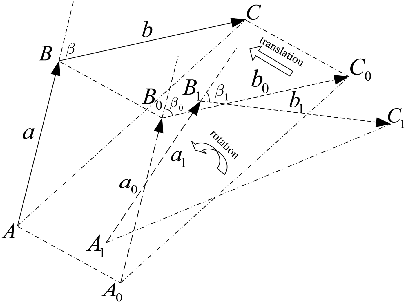
As shown in Figure 1, when the carrier enters into the applicable matching zone, the position and angle information exported by the INS contains accumulative errors, which will result in the position and angle errors between the constructed triangle constraint model and actual triangle. For example, errors of turn angle between the triangle constraint model ΔA1B1C1 and actual triangle ΔABC as well as position errors between the middle transitional triangle ΔA0B0C0 and ΔABC in Figure 3.
Figure 3. Rotation and translation between triangle constraint model and actual triangle.
2.3.1. Definition of measurement parameters of triangle similarity
Because the triangle still maintains similarity after rotation, translation and stretching transformation, the centre of gravity is selected as a triangle rotation centre in this paper. Provided that the triangle ΔA1B1C1 becomes a similar triangle ΔABC after rotation, translation and stretching transformation, then the transformation formula corresponding to coordinates is:
 $$\left[ {\matrix{ {x^i} \cr {y^i} \cr}} \right] = s\left[ {\matrix{ {\cos \phi} & {\sin \phi} \cr { - \sin \phi} & {\cos \phi} \cr}} \right]\left[ {\matrix{ {x_1^i} \cr {y_1^i} \cr}} \right] + \left[ {\matrix{ {t_x} \cr {t_y} \cr}} \right]$$
where (x i, y i) and (x 1i, y 1i)(i = 1,2,3) are respectively coordinates for three angles in ΔABC and ΔA1B1C1, φ is rotation angle (positive in a counter-clockwise direction), s is a scaling coefficient, and (t x, ty) is a translation vector. The similarity matching for two triangles means seeking a group of optimal parameters t x, ty, s, and φ to realise the greatest similarity of two triangles.
2.3.2. Constraint conditions of triangle matching model
In the process of matching for the gravity map as shown in Figure 3, the error factors such as measurement error from gravity map grid resolution and the gravity meter as well as random error of the INS, result in the non-rigid transformation between the triangle constraint model and the triangle matching model. The side lengths of the triangle constraint model come from the relative distances exported from the INS at t i relative to t i−m and t i+k relative to t i, and the relative turn angle at t i, but not including the accumulated errors of the INS. These lengths can be assumed as the “actual values”. So, the constraint conditions for the matching model sides and direction angles are defined in the construction of the triangle-matching model. The matching triangles which are not in line with the triangle-matching model sets can be cropped.
2.3.2.1. Constraint conditions of sides
 $$\vert {P_{1\comma\,i} P_{2\comma\,j} - a}\vert \lt R_a\comma\; \vert {P_{2\comma\,j} P_{3\comma\,k} - b}\vert \lt R_b$$
P 1,i, P 2,j and P 3,k (i, j, k are natural numbers) are points respectively on P 1, P2 and P 3; P1, P2 and P 3 are matching points from the gravity database based on the gravity values measurements; a and b are sides AB and BC for the triangle constraint model respectively; R a and R b are the confidence radius determined in accordance with error source of the non-rigid transformation.
2.3.2.2. Constraint conditions of direction angle
 $$\left( \mathop {AB} \limits^{\rightharpoonup} - \mathop {BC} \limits^{\rightharpoonup} \right) \cdot \left({\mathop {P_{1,i} P_{2,j}} \limits^{\rightharpoonup}} - {\mathop {P_{2,j} P_{3,k}} \limits ^{\rightharpoonup}} \right) \gt 0$$
 $\mathop {AB} ^{\rightharpoonup}$ and
  $\mathop {BC} ^{rightharpoonup} $ are vectors corresponding to two sides of the triangle constraint model.
The modelling analysis and matching calculation can be implemented in accordance with the above triangle constraint conditions.
3. BUILDING AND ACQUISITION OF INITIAL TRIANGLE MATCHING MODEL
See Figure 1. When the carrier enters into the applicable matching area, the position and navigation information provided by the INS in real time contains accumulated errors. In order to quickly and accurately get results of initial matching, the steps to build and get the initial triangle-matching model are:
3.1. Determination of matching and searching area
As shown in Figure 4, a × n2 arrays with equal dimensions (a is the side length of the minimum square area which can be determined by gravity gradient, n is series) shall be established in accordance with carrier position A(x, y) provided in a certain sampling point of the INS. In order to cover the actual track points for the searching area and prevent an endless loop in the process of searching and matching points, the maximum searching series shall be set as N (N depends on the range of accumulative errors when the INS provides the position point A(x, y), and it can be determined by the error and working time of INS), i.e. the maximum searching range is an aN × aN square area.
Figure 4. Searching array for matching points of initial matching process.
3.2. Methods of searching and getting initial matching points
As shown in Figure 5, the square array (including a ij (i = 1,2,3,4; j = 1,2,3,4), which reflects the ith line and jth column square area of Figure 5) refers to the matching searching area at t. g i (i = 1,2,3,4) refers to the contour line with the gravity value of g i in the gravity field. There are numerous position points in each contour line. In order to quickly get the corresponding matching points, the gravity value measured by the gravity meter carried by the carrier at t is assumed as g t in the process of initial matching. Firstly, select the corresponding contour line in the gravity database by the reference value of g t (g 1 and g 4 in Figure 5); secondly, divide the matched contour line into several parts by the unit of array, e.g. a 13, a14, a24, a33, a42 and a 43; thirdly, take the midpoint in the lines corresponding to the contour lines for the array as the matching point, e.g. P ij (i is natural number, j = 1, 2, …, 6).
Figure 5. Searching diagram for initial matching points.
3.3. Building of initial triangle matching model sets
Provided that the INS exports three positions A 1, A2 and A 3 at t i−m, ti and t i+k respectively (m and k are chosen according to the accuracy, and can be the same), then three corresponding and matched searching areas (a uniform 4-level array in Figure 6) as well as initial matching points are obtained at t i−m, ti and t i+k, to form three groups of matching point sets P 1 = {P 11, P12, P13}, P 2 = {P 21, P22, ··· P 26} and P 3 = {P 31, P32, ··· P 39}. Connect each point in the point sets P 1, P 2, P 3 in sequence to build a triangle matching set Ω. The number of possible triangles is  $C_{n1}^1 C_{n2}^1 C_{n3}^1 $ (n 1, n2 and n 3 are numbers of three point sets P 1, P 2, P 3 respectively).
Figure 6. Building of diagram of initial triangle matching model.
3.4. Acquisition of the initial triangle matching model
In order to improve the speed of the initial matching process, the initial triangle matching model set Ω shall be cut in accordance with its constraint conditions to get the initial triangle matching model set Ω′. When the number of triangle matching model in the model set Ω′ is more than one, the 4th position point A 4 exported by the INS shall be continually used, and then the information of three positions A 2, A3 and A 4 will help to build a new triangle matching model until getting the optimal initial triangle matching model.
4. ANALYTICAL METHOD OF TRIANGLE MATCHING PARAMETERS
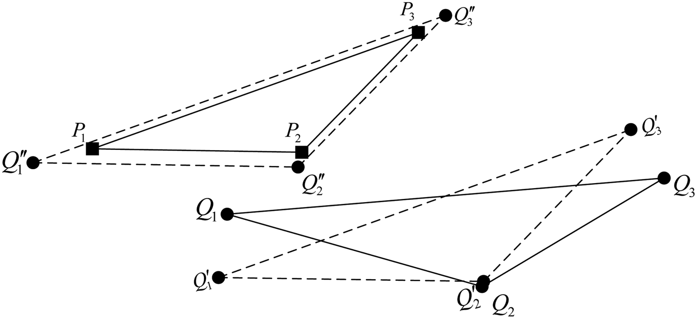
As shown in Figure 7, the triangle constraint model ΔQ 1Q2Q3 and the triangle matching model ΔP 1P2P3 may not be matched with each other completely due to system error or sensor error in the process of the matching algorithm. In this section, the translation and rotation information satisfying the objective triangle matching model will be solved in accordance with the known information about the triangle constraint model.
Figure 7. Rotation and translation transformation of triangles.
Set the three-dimensional matrix R as the rotation matrix from ΔQ 1Q2Q3 to ΔQ′ 1Q′2Q′3 (rotate around the centre of ΔQ 1Q2Q3 counter clockwise).  ${\mathop {t}\limits^{\rightharpoonup}} = \left(t_x\comma\, t_y\comma\, t_z\right)^T$ is the translation vector for the triangle constraint model from ΔQ′ 1Q′ 2Q′ 3 to ΔQ″ 1Q″ 2Q″ 3, and rotation and translation transformation formula for the vector of coordinate point is:
 $$\left[ {\matrix{{x^{\prime}} \cr {y^{\prime}} \cr {z^{\prime}}}} \right] = {\mathop {t} \limits^{\rightharpoonup}} + R \left[ {\matrix{x \cr y \cr z}} \right] + {{\mathop {q} \limits^{\rightharpoonup}} _0}$$
where [x′, y′, z′]T is the vector after translation and rotation, [x, y, z]T is the vector before translation and rotation,  ${\mathop {q}\limits^{\rightharpoonup}}_{0}$ is the centre of ΔQ 1Q2Q3.
Matched objective: The distance square error of the corresponding point is minimum, i.e. the sum of distance square errors between the  $\Delta Q^{\prime\prime}_1 Q^{\prime\prime}_2Q^{\prime\prime}_3 $ after rotation and translation of ΔQ 1Q2Q3 and the corresponding point of ΔP 1P2P3 is minimum. Define the coordinate vector for each point of ΔP 1P2P3 as
  ${\mathop {p}\limits^{\rightharpoonup}}_{i} = \left({\mathop {x} \limits^{\rightharpoonup}}_{\!\!pi}\comma\, {\mathop {y}\limits^{\rightharpoonup}}_{\!\!pi}\comma\, {\mathop {z}\limits^{\rightharpoonup}}_{\!\!pi}\right)^T$,
  ${\mathop {q}\limits^{\rightharpoonup}}_{i} = \left({\mathop {x}\limits^{\rightharpoonup}}_{\!\!qi}\comma\, {\mathop {y}\limits^{\rightharpoonup}}_{\!\!qi}\comma\, {\mathop {z}\limits^{\rightharpoonup}}_{\!\!qi}\right)^T$ for ΔQ 1Q2Q3,
  ${\mathop {q}\limits^{\rightharpoonup}}_{i}^\prime = \left({\mathop {x}\limits^{\rightharpoonup}}_{qi}^\prime\comma\, {\mathop {y}\limits^{\rightharpoonup}}_{qi}^\prime\comma\, {\mathop {z}\limits^{\rightharpoonup}}_{qi}^\prime \right)^T$ for ΔQ′ 1Q′ 2Q′ 3 and
  ${\mathop {q}\limits^{\rightharpoonup}}_{i}^{\prime\prime} = \left({\mathop {x}\limits^{\rightharpoonup}}_{\!\!qi}^{\prime\prime}\comma\, {\mathop {y}\limits^{\rightharpoonup}}_{\!\!qi}^{\prime\prime}\comma\, {\mathop {z}\limits^{\rightharpoonup}}_{\!\!qi}^{\prime\prime} \right)^T$ for ΔQ″ 1Q″ 2Q″ 3. Then the objective function is:
 $$T\left(\mathop {t} \limits^{\rightharpoonup}\comma R \right) = \sum\limits_{i = 1}^3 {\left\Vert{\mathop {p} \limits^{\rightharpoonup}}_i - {\mathop {q} \limits^{\rightharpoonup}}_i^{\prime\prime}\right\Vert}^2$$
Meanwhile, the rotating translation formula for the triangles from ΔQ 1Q2Q3 to ΔQ″ 1Q″ 2Q″ 3 is:
 $${q_i^{\prime\prime}} = R\left({{\mathop {q} \limits^{\rightharpoonup}}_i}^\prime - {\mathop {q} \limits^{\rightharpoonup}}_0 \right) + \mathop {t} \limits^{\rightharpoonup} + {\mathop {q} \limits^{\rightharpoonup}}_0$$
The final objective function is:
 $$T\left(\ \mathop {t}\limits^{\rightharpoonup}\comma\, R \right) = \sum\limits_{i = 1}^3 {\left\Vert{\mathop {\,p}\limits^{\rightharpoonup}}_{i} - R\left({{\mathop {q}\limits^{\rightharpoonup}}_{i}}^\prime - {\mathop {q} \limits^{\rightharpoonup}}_{0} \right) - \mathop {t}\limits^{\rightharpoonup} -\, {\mathop {q} \limits^{\rightharpoonup}}_{0}\right\Vert}^2$$
Because there is no relationship between translation vector  $\mathop {t}\limits^{\rightharpoonup}$ and rotation matrix R, it can be calculated separately to get the minimum value for the objective function.
4.1. Calculation method of translation vector
The translation vector  $\mathop {t}\limits^{\rightharpoonup}$ shall satisfy the following conditions to get minimum value for the objective function:
 $${\displaystyle{\partial T \left(\ \mathop {t}\limits^{\rightharpoonup} \comma\, R \right)} \over {\partial\, {\mathop {t}\limits^{\rightharpoonup}}}} = 0$$
While
 $${\displaystyle{\partial T \left(\mathop {t}\limits^{\rightharpoonup} \comma\, R \right)} \over {\partial\, {\mathop {t}\limits^{\rightharpoonup}}}} = \left[ {\displaystyle{{\partial T} \over {\partial t_x}} \comma \displaystyle{{\partial T} \over {\partial t_y}} \comma \displaystyle{{\partial T} \over {\partial t_z}}} \right]^T$$
Then
 $$\displaystyle{{\partial T} \over {\partial t_{\rm j}}} = 0 \comma\, ({\rm where}j = x \comma\, y \comma\, z)$$
Select a group of orthogonal basis {ex, ey, ez}, where ex = (1,0,0)T, ey = (0,1,0)T, and ez = (0,0,1)T
 $$\eqalign{\displaystyle{{\partial T} \over {\partial t_j}} & = {\displaystyle{\partial\left\{\sum\limits_{i = 1}^3 {\left\Vert{\mathop {\,p}\limits^{\rightharpoonup}}_{i} - R\left({{\mathop {q}\limits^{\rightharpoonup}}_{i}}^\prime - {\mathop {q}\limits^{\rightharpoonup}}_{0} \right) - \mathop {t} \limits^{\rightharpoonup} -\, {\mathop {q}\limits^{\rightharpoonup}}_{0} \right\Vert}^2\right\} \over {\partial t_j}}} \cr & = -2{\left[\sum\limits_{i = 1}^3 {\bf e}_j^T \left({{\mathop {\,p}\limits^{\rightharpoonup}}_{i} - R\left({{\mathop {q}\limits^{\rightharpoonup}}_{i}}^\prime - {\mathop {q}\limits^{\rightharpoonup}}_{0} \right) - \mathop {t}\limits^{\rightharpoonup} -\, {\mathop {q}\limits^{\rightharpoonup}}_{0}}\right)\right]}}$$
So
 $$\displaystyle{{\partial T} \over {\partial t_j}} = -2{\left[\sum\limits_{i = 1}^3 {\bf e}_j^T \left({{\mathop {\,p}\limits^{\rightharpoonup}}_{i} - R\left({{\mathop {q}\limits^{\rightharpoonup}}_{i}}^\prime - {\mathop {q}\limits^{\rightharpoonup}}_{0} \right) - \mathop {t}\limits^{\rightharpoonup} -\, {\mathop {q}\limits^{\rightharpoonup}}_{0}}\right)\right]} = 0$$
Then value of the translation vector  $\mathop {t}\limits^{\rightharpoonup}$ is:
 $$\mathop {t}\limits^{\rightharpoonup} = {\displaystyle{1 \over 3}}{\sum\limits_{i = 1}^3 \left({{\mathop {\,p}\limits^{\rightharpoonup}}_{i} - R\left({{\mathop {q}\limits^{\rightharpoonup}}_{i}}^\prime - {\mathop {q}\limits^{\rightharpoonup}}_{0} \right) - {\mathop {q}\limits^{\rightharpoonup}}_{0}}\right)}$$
4.2. Calculation method of rotation matrix
Define  ${\tilde{\mathop {p}\limits^{\rightharpoonup}}_{i}} = {{\mathop {p}\limits^{\rightharpoonup}}_{i}} - {\mathop {t}\limits^{\rightharpoonup}} - {\mathop {q}\limits^{\rightharpoonup}}_{0} = {{\mathop {p}\limits^{\rightharpoonup}}_{i}}- {\mathop {p} \limits^{\rightharpoonup}}_0$,
 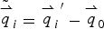 ${\tilde{\mathop {q}\limits^{\rightharpoonup}}_{i}} = {{\mathop {q}\limits^{\rightharpoonup}}_{i}}^{\prime} - {{\mathop {q}\limits^{\rightharpoonup}}_{0}}$, then
 $$\eqalign{T\left(\, \mathop {t}\limits^{\rightharpoonup},R \right) & = {\sum\limits_{i = 1}^3 {\left\Vert{\mathop {\,p}\limits^{\rightharpoonup}}_{i} - R\left({{\mathop {q}\limits^{\rightharpoonup}}_{i}}^\prime - {\mathop {q}\limits^{\rightharpoonup}}_{0} \right) - \mathop {t}\limits^{\rightharpoonup} -\, {\mathop {q}\limits^{\rightharpoonup}}_{0} \right\Vert}^2} \cr & = {\sum\limits_{i = 1}^3 {\left\Vert{\mathop {\,p}\limits^{\rightharpoonup}}_{i} - \mathop {t}\limits^{\rightharpoonup} -\, {\mathop {q}\limits^{\rightharpoonup}}_{0} - R\left({{\mathop {q}\limits^{\rightharpoonup}}_{i}}^\prime - {\mathop {q}\limits^{\rightharpoonup}}_{\!0} \right) \right\Vert}^2}\cr & = {\sum\limits_{i = 1}^3 {\left\Vert\left({\mathop {\,p}\limits^{\rightharpoonup}}_{i} - {\mathop {\,p}\limits^{\rightharpoonup}}_{0}\right ) - R\left({{\mathop {q}\limits^{\rightharpoonup}}_{i}}^\prime - {\mathop {q}\limits^{\rightharpoonup}}_{0} \right) \right\Vert}^2} \cr & = \sum\limits_{i = 1}^3{\left\Vert{\tilde{{\mathop {\,p}\limits^{\rightharpoonup}}}_{i}} - {R\ {\tilde{\mathop {q}\limits^{\rightharpoonup}}}_{i}}\right\Vert}^2 \cr & = \sum\limits_{i = 1}^3\left({\left\Vert{\tilde{{\mathop {\,p}\limits^{\rightharpoonup}}}_{i}}\right\Vert}^2 + {\left\Vert{{\tilde{\mathop {q}\limits^{\rightharpoonup}}}_{i}}\right\Vert}^2 - 2{\tilde{\mathop {\,p}\limits^{\rightharpoonup}}_{i}}^T R\,{\tilde{\mathop {q}\limits^{\rightharpoonup}}_{i}}\right)}$$
 Respectively define 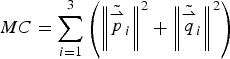 $MC = \sum\limits_{i = 1}^3 \left({\left\Vert{\tilde{\mathop {p}\limits^{\rightharpoonup}}_{i}}\right\Vert}^2 + {\left\Vert{\tilde{\mathop {q}\limits^{\rightharpoonup}}_{i}}\right\Vert}^2\right)$,
 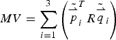 $MV = \sum\limits_{i = 1}^3 \left({\tilde{\mathop {p}\limits^{\rightharpoonup}}_{i}}^T R{\tilde{\mathop {q}\limits^{\rightharpoonup}}_{i}}\right) $, then
 $$T\left(\, \mathop {t}\limits^{\rightharpoonup},R \right) = MC - 2MV$$
Because MC is constant, the maximum MV shall be calculated when the objective function is minimum.
 $$MV = \sum\limits_{i = 1}^3 \left[{\tilde{\mathop {\,p}\limits^{\rightharpoonup}}_{i}}^T R\,{\tilde{\mathop {q}\limits^{\rightharpoonup}}_{i}}\right] = \sum\limits_{i = 1}^3 \left[Trace\left({\tilde{\mathop {\,p}\limits^{\rightharpoonup}}_{i}} \ {{\tilde{\mathop {q}\limits^{\rightharpoonup}}_{i}}}^T R^T\right)\right]$$
 When 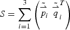 $S = \sum\limits_{i = 1}^3 \left({\tilde{\mathop {p}\limits^{\rightharpoonup}}\!_i} \,\,{{\tilde{\mathop {q}\limits^{\rightharpoonup}}_{i}}}^T\right) $, then
 $$\eqalign{MV & = \sum\limits_{i = 1}^3 \left[Trace\left({\tilde{\mathop {\,p}\limits^{\rightharpoonup}}_{i}}\, {{\tilde{\mathop {q}\limits^{\rightharpoonup}}_{i}}}^T R^T\right)\right] \cr & = Trace \left[\sum\limits_{i = 1}^3\left({\tilde{\mathop {\,p}\limits^{\rightharpoonup}}_i}\ {{\tilde{\mathop {q}\limits^{\rightharpoonup}}_i}}^T \right)R^T\right] = Trace\left(SR^T \right)}$$
The Singular Value Decomposition (SVP) for S shall be S = UWV T, where U and V are orthogonal matrices, and W = diag(w 1, w 2, w 3), w i ≥ 0, then
 $$\eqalign{Trace\left( {SR^T} \right) & = Trace\left( {UWV^T R^T} \right) \cr & = Trace\left( {UWV^T R^T UU^T} \right) = Trace\left( {WV^T R^T U} \right)}$$
Meanwhile, let Z = V TR TU, and the matrix Z is also the orthogonal matrix as U, V and R are orthogonal matrices, then
 $$Trace\left( {SR^T} \right) = Trace\left( {WV^T R^T U} \right) = Trace\left( {WZ} \right) \le Trace\left( W \right)$$
Only when Z = V TR TU = I, can Trace(SR T) achieve the maximum value, i.e. MV achieves the maximum value, and the objective function  $T\left(\,\mathop {t}\limits^{\rightharpoonup} \comma\, R \right)$ has the minimum value. Then the calculation formula of the rotation matrix R is:
 $$R = UV^T $$
4.3. Measurement method of triangle similarity
The normalisation mapping of the triangle can be implemented in accordance with its stretching feature in order to conduct the similarity measurement of the triangle, and the mapping function for the normalisation is:
 $$\eqalign{& (x,y) = f\,(a,b,c) \cr & x = \displaystyle{a \over {\rm c}} \comma\,\, y = \displaystyle{b \over c}{(\hbox{Assume c to be the longest between the three sides a, b, c of a triangle} )}} $$
See Figure 8. Define three sides of ΔQ 1Q 2Q 3 as Q 1Q 2 = a q, Q 2Q 3 = b q and Q 1Q 3 = c q respectively, and three sides for ΔP 1P 2P 3 as P 1P 2 = a p, P 2P 3 = b p and P 1P 3 = c p respectively. So the two triangles are mapped as one point on the plane, and the data range of this point is [0, 1].
Figure 8. Principle of triangle normalisation mapping.
Select the relative errors ε x, ε y of the mapping points to get the similarity of two triangles. Define P′(x p, y p) and Q′(x q, y q), then
 $$c = 1 - f\,(\varepsilon _x \comma\, \varepsilon _y )$$
Where
 $$f\,(\varepsilon _x \comma\, \varepsilon _y ) = \sqrt {\displaystyle{{\varepsilon _x^2 + \varepsilon _y^2} \over 2}}$$
While
 $$\varepsilon _x = 2\displaystyle{{x_p - x_q} \over {x_p + x_q}} \comma\, \varepsilon _y = 2\displaystyle{{y_p - y_q} \over {y_p + y_q}}$$
Based on calculation of the Euler distance between two points in the mapping space, the distance can be taken as a similarity measurement parameter for two corresponding triangles as well as a reliable evaluation parameter for matching results of the triangle-matching algorithm.
5. SIMULATION ANALYSIS OF PRECISION FOR INITIAL MATCHING
5.1. Design of simulation platform
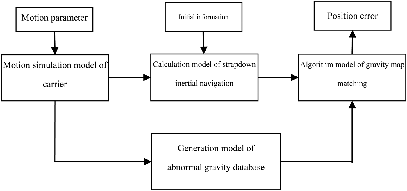
To conduct simulation analysis on the initial matching technical precision of the triangle constraint model, this paper establishes a simulation platform based on Matlab, mainly including a motion simulation model of the carrier, a generation model of abnormal gravity database, a calculation model of strapdown inertial navigation and the algorithm model of gravity map matching (see Figure 9).
Figure 9. Schematic diagram of simulation platform module.
5.1.1. Motion simulation model of carrier
The motion model of the carrier applies the six-variable fluid mechanical models in Healay and Lienard (Reference Healay and Lienard1993) and Li et al. (Reference Li, Bian and Shi2007), and the six variables are the average speed and angular velocity in the front, right and bottom of the self-system respectively, and they are also the expression of the self-system relative to the ocean current. They are expressed as:
 $$x(t) = [u(t) \comma\, v(t) \comma\, \omega (t) \comma\, p(t) \comma\, q(t) \comma\, r(t)]$$
where u(t), v(t), ω (t) are average speed in the front, right and bottom of the self-system and p(t), q(t), r(t) are angular velocity in the front, right and bottom of the self-system.
This paper mainly transforms the quantities into an expression of the self-system relative to the ocean current in the ocean current system, and then changes them into the position and attitude information of the self-system relative to the navigation system.
5.1.2. Generation model of abnormal gravity database
This refers to the range of global abnormal gravity changes, and determines the simulation data range of abnormal gravity between −80mGal to 80mGal (1mGal ≈ 10−5m/s 2). The random numbers are generated as follows: Firstly, generate a 3 × 3 random number with Matlab, and enable them to present a normal distribution at [0, 60mGal]; secondly, generate nine 3 × 3 random numbers by the centre of each random number, and enable them to present a normal distribution at [0, 20mGal]; add them to the centre data, and get a 9 × 9 database; thirdly, generate 81 3 × 3 random numbers by the centre of each 9 × 9 random number, and enable them to present a normal distribution at [0, 5mGal]; then add them to the centre data and get a 27 × 27 database; finally, generate several 50 × 50 random numbers by the centre of each 27 × 27 random number and enable them to present a normal distribution at [0, 5mGal]; then add them to the centre data, and get a 1350 × 1350 random database, which shall be disposed smoothly to be the final abnormal gravity database.
Figure 10 shows the simulated abnormal gravity database which corresponds to a longitude range of 115° − 117·7° and a latitude range of 38° − 40·7°. The resolution ratio of its longitude and latitude grid is 0·002°/grid.
Figure 10. Simulation of local abnormal gravity database. (a) Three-dimensional gravity field (b) Contour map.
5.1.3. Realisation of dynamic analogue simulation
5.1.3.1. Simulation of measurement value for gravity meter
The samples are taken in the abnormal gravity database in accordance with actual traces of the simulated carrier, and the 0·05 mGal white noise is superposed in the sampling data to simulate the measurement value of the gravity meter in real time with a sampling period of 150 s.
5.1.3.2. Simulation of dynamic trace for real-time export carrier of INS
The dynamic trace simulation model of the carrier offers its real position and attitude information, then generates the output of the inertial device (gyroscope and weight) based on the position and attitude information. Meanwhile, it overlays the random drift of accelerometer, random zero offset of the gyroscope and white noise. Finally the position information with errors is obtained by the inertial navigation calculation as the actual trace of the carrier, where the carrier's quality is assumed to be 5454·5 kg, and its route speed is 40 knots (about 74 km/h). The suitable matching area of the gravity map is the one covered by the simulated abnormal gravity database. In addition, the accumulated errors (i.e. initial error of INS) for the suitable-matching area of the gravity map for the INS can be acquired directly by overlaying the constant value.
5.2. Simulation analysis of initial matching precision
5.2.1. Simulation analysis of initial matching precision for short endurance
Before access to the gravity suitable matching area, the accumulated longitude and latitude errors for the INS shall be set as 0·01°, the drift error of the constant value as 0·01°/h, and the random noise as 0·001°.
Figures 11 (a) and (b) show the local magnification diagram of matching results for the previous ICCP algorithm and triangle algorithm respectively, and Figures 11 (c) and (d) show the longitude and latitude matching error diagrams respectively. It is known from the above figures that the matching precision of the triangle-matching algorithm on the first matching point is higher than that of the ICCP algorithm. However, the precisions of two algorithms are equivalent, while the matching error decreases in the matching process.
Figure 11. Comparison of matching results for short endurance.
5.2.2. Simulation analysis of error model for long endurance
Before access to the gravity suitable matching area, the accumulated longitude and latitude errors for the INS shall be set as 0·05°, the drift error of the constant value as 0·01°/h, and the random noise as 0·001°.
Figure 12 shows the matching traces and longitude-latitude matching errors for the ICCP and triangle algorithms. For the triangle-matching algorithm, the precision of initial matching at an initial error 0·05° for the long endurance is more obvious than the matching result that the initial error is 0·01° for the short endurance. The precision of initial matching corresponding to the triangle-matching algorithm for the long endurance is three and four times higher than that of the ICCP algorithm, nearly up to the overall matching precision.
Figure 12. Comparison of matching results for long endurance.
Figure 13 shows the comparison of calculating time consumption between the ICCP algorithm and the triangle algorithm for simulation by Matlab. It is known from the figure that the main reason why the time-consuming vibration corresponding to each matching point is larger is that the iterations of the ICCP algorithm are uncertain. Low or high matching precision for the first time results in different iterations, and even time-consuming vibration effects. Moreover, the general time consumption of the ICCP algorithm increases with sequence points. The reason for this is that the increase of matching sequence points results in a linear growth of time consumption for the matrix operation. Compared with the ICCP algorithm, the time consumption of the triangle-matching algorithm is relatively steady because each matching operation only needs three sequence points in the matrix operation rather than the iteration operation. In this way, the time consuming stability of the triangle-matching algorithm is ensured.
Figure 13. Comparison of time-consumption between triangle and ICCP algorithms. (a) short endurance (b) long endurance.
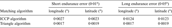
Table 1 provides longitude and latitude error results respectively corresponding to the short and long endurances, and the calculation method is useful to high precision GNSS differential results as a benchmark and to calculate the average value of all matching errors.
Table 1. Comparison of simulation errors between triangle and ICCP algorithms.
From the table, the initial longitude and latitude error of the inertial navigation is 0·01° or 0·05°, and the matching error of the triangle-matching algorithm shall be maintained within 0·002° (about 220 m). When the initial error of inertial navigation for the ICCP algorithm is 0·01°, the matching error is close to 0·002°; when it is 0·05°, the matching error exceeds 0·01° (about 1100 m). Generally, the ICCP algorithm is more sensitive to the initial error which will directly affect the matching results. While the matching algorithm of the triangle constraint model is not sensitive to the initial error and can effectively overcome different initial errors, so the longitude and latitude error of the inertial navigation can be decreased by 20% below the random drift.
6. SIMULATION COMPARISON
Three groups of simulations were implemented in the Bohai Sea, South China Sea and Pacific Ocean respectively, in order to compare the triangle matching algorithm with the prevalent ICCP algorithm. The simulation conditions are as follows:
(1) The INS initial error (Lon/deg, Lat/deg) ranges from 0·050–0·010 and 0·0020 in each group.
(2) The drift error of the INS constant value is 0·010/h, and the random noise is 0·0010.
(3) The gravimeter is simulated by sampling the gravity data from the gravity field maps along the Autonomous Underwater Vehicle (AUV) path and adding the gravity noise regardless of the influence from waves and current. The gravity noise, which mainly reflects the precision of the simulated gravimeter occurs in the normal distribution at a variance of 0·01 mGal, and the time for sampling is 150 seconds.
(4) The grid resolution of the original gravity field maps, which are provided by the Scripps Institution of Oceanography, is just 0·0160 per grid. The original gravity field maps are defined to 0·0020/grid by the Kriging algorithm.
(5) Motion simulation model of carrier makes the trace of the carrier.
(6) The speed of the AUV is 60 km/h, the time for sampling is 150 seconds, and all the simulations will be implemented for 3600 seconds.
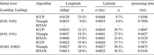
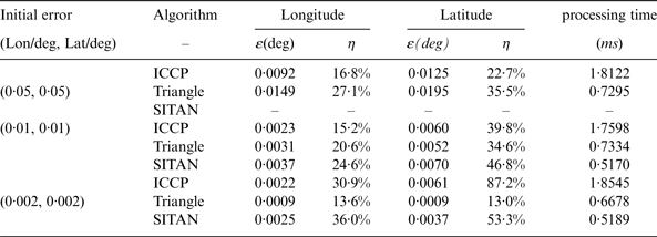
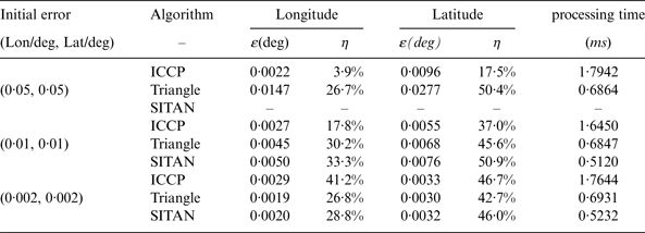
In Tables 1 and 2, the remainder error ε(deg) = |e 1–e2| represents the difference between the added position error e 1 and the matching result e 2 in degrees, and η = ε/e 1 is the percentage of the remainder error ε (°) related to the added position error. It is important to note that the results given in the tables are all mean values, as are the yaw error (°), reliability (%), and processing time (ms) respectively for each point.
Table 2. Simulation results in the Bohai Sea local district.
From the simulation results in Tables 2 to 4 and Figures 14 to 16, the SITAN algorithm cannot provide matching results when the initial error is larger (the initial longitude and latitude errors in this paper are all set as 0·05°); when the initial error gradually decreases from 0·01° to 0·002°, the residual error of the SITAN algorithm ε (°) gradually decreases, and the corresponding relative residual error η can remain an acceptable result.
Figure 14. Gravity fieldmap in Bohai Sea local district and the actual path.
Figure 15. Gravity field map in South China Sea local district and the actual path.
Figure 16. Gravity field map in Pacific Ocean local district and the actual path.
Table 3. Simulation results in the South China Sea local district.
Table 4. Simulation results in the Pacific Ocean local district.
From the comparison and analysis results of ICCP, SITAN and triangle matching algorithms in Tables 2 to 4, the matching precision of the triangle matching algorithm is equivalent to that of the ICCP algorithm under the larger initial error for inertial navigation, but the triangle matching algorithm has better real-time level; when the initial error of the inertial navigation is smaller, both triangle matching and SITAN algorithms have equivalent real-time level.
7. CONCLUSIONS
In the case of large initial errors, the matching algorithm based on the triangle gives the results of the initial matching accuracy quickly and effectively. In the whole matching process, the errors introduced by non-rigid transformation are considered in the triangle-matching algorithm, which is of great flexibility and high precision. In addition, the single matching is stable in a triangle-matching algorithm with a small amount of computation.
The triangle-matching algorithm can be applied independently in conjunction with an ICCP algorithm or the SITAN algorithm. When the carrier enters into the suitable-matching area, accurate initial matching algorithm parameters are obtained for the ICCP and SITAN algorithms.
ACKNOWLEDGEMENTS
The authors thank the Scripps Institution of Oceanography and the University of California San Diego for providing the original gravity field maps. The work reported here has been supported by the Foundation for Innovative Research Groups of the National Natural Science Foundation of China under a grant number of 61121003, by MOST Major Scientific Equipment Special of China under a grant number of 2012YQ160185.