


Introduction
An extensive data base on topographic glacier parameters has been built up in regional glacier inventories (Haeberli and others, 1989). Repetition of such glacier inventory work is planned at time intervals comparable to the characteristic dynamic response times of mountain glaciers (a few decades). This should help with analyzing changes at a regional scale and with assessing the representativeness of continuous measurements which can only be carried out on a few selected glaciers. In addition, glacier inventory data serve as a statistical basis for extrapolating the results of observations or model calculations concerning individual glaciers (Reference Oerlemans and PeltierOerlemans, 1993,Reference Oerlemans1994) and to simulate regional aspects of past and potential climate-change effects. This latter application requires the introduction of a parameterization scheme using simple algorithms for unmeasured glaciers. A corresponding scheme is explained and illustrated with the example of the European Alps. The procedure described also enables plausibility checks to be carried out on the large sample of inventory data and is presently being systematically applied while loading available detailed inventories into the new data bank of the World Glacier Monitoring Service (WGMS) (paper in preparation by Reference Hoelzle and Trindler.M. Hoelzle and M. Trindler).
Parameterization Scheme
The basis for the parameterization scheme (cf. Reference HoelzleHoelzle (1994) for more detailed discussion) consists of measured inventory data on the total length (L 0), maximum/minimum altitude (H max, H min) and total surface area [F] of the investigated glaciers. From these basic parameters, mean altitude (H m = [H max – H min]/2), vertical extent (ΔΗ = H max – H min) and average surface slope (α = arctan[ΔH/L 0]) are derived as a first step. The length of the central flowline in the ablation area (L a) is empirically set as 0.5L 0 (Reference MüllerMüller, 1988) for glaciers ≤2km, and as 0.75L 0 for glaciers > 2 km. The mean slope of the ablation area (α a) is then computed from arctan(H m – H min)/L a. Average ice depth along the central flowline (h f) is estimated from α and a mean basal shear stress along the central flowline (τ f = f ρgh f sin α, where ρ is density and g is acceleration due to gravity) which depends in a non-linear way on ΔH as a function of mass turnover (Fig. 1; cf. Reference HaeberliHaeberli, 1985; Reference Driedger and Kennard.Driedger and Kennard, 1986). The shape factor f is chosen as 0.8 for all glaciers. Ice thickness in the ablation area (h f,a) is derived from τ f and α a and maximum thickness (h max) is very roughly determined at 2.5h f,a, as estimated from known ice thickness measurements on various Alpine glaciers (Reference Müller, Caflisch and Müller.Müller and others. 1976; unpublished radio-echo soundings/hot-water drillings by VAW/ETH Zürich) and in order to account for sonic longitudinal variations in α. Average thickness of the entire (three-dimensional) glacier is assumed to be h F = (π/4)h f in accordance with a semi-elliptic cross-sectional geometry. Total glacier volume then becomes V = Fh F.

Fig. 1. Average basal shear stress along the central flowline vs altitudinal extent of (reconstructed late-Pleistocene Alpine) glaciers (modified from Haeberli (1985)). The polynomial fit gives the function used in the present study. A maximum value of 1.5 bar (150 kPa) was assumed for the largest glaciers.
Mean altitude (H m) is taken as an approximation for equilibrium-line altitude (ELA; cf. Reference Braithwaite and Mü;ller.Braithwaite and Müller, 1980), and the mass balance (annual ablation) at the glacier tongue is computed as b t = db/dH (H m – H min) where the mass-balance gradient db/dH receives a value of 0.75 m w.e. per 100 m and year for the ablation area, as appears quite characteristic for the Alps (Reference Oerlemans and Hoogendorn.Oerlemans and Hoogendorn, 1989; Reference Oerlemans and Fortuin.Oerlemans and Fortuin, 1992). Depth-averaged mean flow velocity along the central flowline in the ablation area is calculated as balance velocity for the lower half of the ablation area as u m,a = [(3b t/4)(La/2)]/hf,a. For simplicity, the corresponding surface flow velocity u s,a is assumed not to differ significantly from u m,a; its component of ice deformation is calculated from u d,a = 2Ατ f n h f/(n + 1) where A is uniformly chosen as 0.16 a−1 bar−3 and n = 3 to give realistic values (cf. Reference PatersonPaterson, 1981). The combined consideration of mass conservation and the ice-flow law would, in principle. allow the sliding velocity in the ablation area to be estimated as u b,a = u s,a. The velocity ratio in the ablation area would then be defined as u b,a/u s,a. In view of the limited data base and the uncertainties involved with the flow-law parameters, however, firn conclusions cannot be expected from such dynamic considerations.
Glacier-length changes [δL = L 0 δb/b t ; cf. Reference PatersonPaterson, 1981; Reference Haeberli and BenistonHaeberli, 1994) for given disturbances in mass balance (δb) are calculated with reaped to the characteristic dynamic response time t resp = h max/b t (cf. Reference Jóhannesson, Raymond and Waddington.Jóhannesson and others, 1989) in the sense of step functions between steady-state conditions. The reaction time between the onset of δb and the first reaction at the glacier terminus is estimated as t react = L a/c, where c is the kinematic wave velocity (Reference NyeNye, 1965). The application of kinematic wave theory is especially delicate (Reference Lliboutry and Reynaud.Lliboutry and Reynaud, 1981), but the reaction times calculated with c = 4u s.a seem to compare quite well with observed advance patterns (Reference MüllerMüller, 1988). The time interval between the first reaction at the glacier terminus and full response to δb is called relaxation time (paper in preparation by T. J.H. Chinn): t relax = t resp – t react.
Near-surface thermal regime (10 m temperature) is defined from empirical relations between mean annual air, firn and ice temperatures (Reference Haeberli and Alean.Haeberli and Alean, 1985) in the following way: cold firn is believed to exist everywhere above the −12°C mean annual air-tempera in re isotherm, and ablation areas are expected to be partially cold where mean annual air temperature at the ELA (H m) is below – 4°C. This first-order approach could be improved by using a relation between 10 m ice and mean summer air temperatures (Reference Hooke, Gold and Brzozowski.Hooke and others, 1983).
Present-Day Glacierization
The data for the European Alps as used in the present study and containing a total of 5050 perennial surface ice bodies were compiled for the mid-1970s (Austria 1969, France 1967–71, Germany 1979, Italy 1975–84, Switzerland 1973). Only 1763 of these ice bodies (35%) are glaciers larger than 0.2 km2 with complete information available about surface area, total length and maximum and minimum altitude. The above-explained parameterization scheme is applied to this part of the sample. The remaining 3287 ice bodies (65% are perennial ice patches and glacierets smaller than 0.2 km2 and are treated separately.
The total surface area of all 5050 inventoried surface ice bodies is 2909 km2 (Haeberli and others, 1989). The surface area of the 1763 glaciers > 0.2 km2 is 2533 km2, or 88% of the total surface area. The total volume of these glaciers > 0.2 km2 is calculated as 126 km3, that of the 3287 glacierets ≤ 0.2 km2 as 2.6 km3. The Latter value is globally estimated by taking half (7.5 m) in the mean value of h F (15 ± 4 m) for glaciers with 0.2< F < 0.4 km2. The overall volume of perennial surface ice in the Alps around 1970 is thus about 130 km3. Complete melting of this ice volume would cause a sea-level rise of about 0.35 mm. Such a small value is not of great importance for sea-level rise lint suggests the vulnerability to climate effects of glaciers in comparable high mountain areas with predominantly small glaciers. The decade 1980–90 with a mean annual mass balance of −0.65 m w.e. as measured on eight regularly observed glaciers in the Alps (Caréser, Gries, Hintereis, Kesselwand, Saint Sorlin, Sarermes, Silvretta, Sonnblick; Reference Haeberli and Mü;ller.Haeberli and Müller, 1988; Reference Haeberli and Hoelzle.Haeberli and Hoelzle, 1993; cf. Reference Haeberli and BenistonHaeberli, 1994) may have brought about a loss in surface ice volume of nearly 20 km3 or about 10–20% of the total volume existing around 1970. It is reasonable to assume that the total volume of perennial Alpine surface ice is now (1994) not much higher than 100 km3. Comparably low total glacier volumes may have existed around 1950AD, around 4000 BP and around 5000 BP; even smaller ice volumes can possibly be attributed to the early Holocene, i.e. the time period around 7000–6000 BP (Reference Haeberli and BenistonHaeberli, 1994)
A number of interesting glaciological characteristics can also be derived with respect to the investigated sample of Alpine glaciers (Fig. 2). Only 54 (3%) of the 1763 glaciers > 0.2 km2 begin above 4000 m a.s.l. and. hence, definitely have parts of cold firn in their accumulation areas. On the other hand, 1323 (75%) of all glaciers > 0.2 km2 have ELAs (mean altitudes) above 2800 m a.s.l., where mean annual air temperature is around −4°C. This means that for the most part the Alpine glaciers are not strictly temperate but rather poly thermal with more or less extended cold parts (surface layers) in their ablation areas. Most glaciers (88%) have mean annual air temperatures at the equilibrium line between −2° and −6°C (2500 ≤ H m ≤ 3200), indicating transitional climatic conditions as opposed to maritime (> −2°C, 2%) and continental (< −6°C, 10%) types of glaciers (cf. Reference HaeberliHaeberli, 1983). More than four out of five glaciers (83%) end above 2400 m a.s.l., i.e. in the altitudinal belt where discontinuous permafrost regularly occurs. More than 90% of the glaciers > 0.2 km2 have total surface areas smaller than 10 km2, lengths shorter than 5 km and overall slopes steeper than 10°. This means that the sample of presently existing Alpine glaciers is dominated by small and steep mountain glaciers with average thicknesses of a few tens of metres. About 70% of these small mountain glaciers have average basal shear stresses along the central flowline which remain below 1 bar (100 kPa). Such rather static ice bodies, called “glaciers réservoirs” by Lliboutry (unpublished), react through (vertical) surface altitude changes rather than pronounced (horizontal) advance/retreat as can be typically observed for the more dynamic, rapidly flowing “glaciers vacuateurs” with higher basal shear stresses (> 1 bar, or > 100 kPa). Calculated surface velocities in the ablation areas of the small mountain glaciers are typically a few tens of metres. Response limes centre around a few decades and are a strongly non-linear function of surface slope (Fig. 3). This result is mainly related to the parameterization applied in the present study but could also be physically reasonable: with slope decreasing towards the horizontal, the difference between equilibrium-line and terminus altitudes (here: H m – H min) and. hence, ablation at the terminus tends to become zero and the response time tends to become indefinitely long because a non-flow condition is being approached. On the other hand, slopes increasing towards the vertical reduce maximum thickness to zero and asymptotically shorten response times towards zero. In such cases, mass transfer on steep to vertical walls is by instabilities and falling of snow and ice rather than by steady ice flow. Reaction lime varies from a few years to a few decades and tends to be one-third to two-thirds of the response time, the higher fraction being more characteristic for the smaller glaciers. Derived relaxation time has a peak frequency around 10 years with decreasing probabilities for longer time intervals.

Fig. 2. Frequency distribution of (a) highest glacier elevation H max. (b) mean glacier elevation H m , (c) lowest glacier elevation H min, (d) glacier area F, (e) average surface slope α, (f) average basal shear stress along the central flowline τ f, (g) balance velocity in the ablation area u m,a and (h) response lime t resp for the glaciers > 0.2km 2 as defined in the text..

Fig. 3. Response times tresp as a function of average surface slope α for glaciers longer than 2 km.
Simulation of Climate-Change Effects
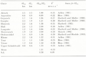
A first experiment was run to simulate maximum glacier extent around 1850 AD, the end of the “LittleIce Age” in central Europe, in order to check how realistic the proposed scheme is as compared to observed long-term changes and then to simulate changes that have happened since. The considered time interval is 120–130 years. In view of the fact that Alpine glaciers remained quite unchanged between 1890 and 1925 (Reference PatzeltPatzelt and Aellen, 1990), the time interval since the middle of the past century spans about twice the characteristic mean response time of the investigated sample of Alpine glaciers. Instead of calculating two subsequent steps with increasing uncertainties about the parameters involved (for instance, ablation at the glacier tongue in times lacking measurements), one single step with a positive mass-balance (step) change of 1 m a−1 was assumed for the entire time interval. This procedure corresponds to a calculation with two steps assuming two full dynamic responses (for instance, 1850–1900 and 1930–80) to a step change in mass balance of 0.5 m a−1 and an average balance of 0.25 m a−1 for both partial intervals. The comparison between calculated and measured length changes for selected glaciers (Table 1) shows that the different sensitivities of long-term glacier length as a response to uniform mass-balance forcing can be quite well reproduced (cf., for instance. Upper Grindelwald and Aletsch) and that the chosen mass-balance forcing appears to underestimate slightly the real evolution. Differences between measured and calculated overall length change for individual glaciers, on the other hand, can be considerable and are explained by uncertainties in the simple parameterization scheme applied, by the limited data base available for each glacier in inventories, and by variable climate/mass-balance conditions at each glacier. Correcting the mass-balance forcing for each glacier to fit the measured length change gives an average mass balance of 0.33±0.09 m a−1 average (secular) mass loss for the sample of glaciers considered in Table 1. If the time period 1850–1970 is treated as one single retreat period without consideration of the 35 years of stationary glaciers, the above calculated value reduces to an average mass loss of 0.2–0.3 m w.e.a−1 The energy required for melting this amount of ice during the time interval 1850–1970 AD is 2–3 W m−1. Such values roughly correspond to the observed long-term trend of atmospheric warming and could be quite representative of (non-polar?) mountain glaciers all over the world (Reference OerlemansOerlemans, 1994).
Table 1. Measured and calcula led cumulai ire length changes and average mass balances of selected Alpine glaciers since 1850 AD. δL m, measured cumulative length change. 1850 – 1970 AD; δL c, calculated total length change. 1850–90 and 1925–70 with a mean mass balance of −0.25 m w.e.a for both partial time intervals; b*, average mass balance. 1850–90 and 1925–70 as corrected by δL m/δL c for the measured length change.
The calculated length change divided by two relaxation times for the two periods considered gives characteristic average rates of length change during marked advance/retreat periods of a few tens of meters per year with steep/high-stress glaciers such as Bionnassey, Taconnaz, Bosson, Breuva, Miage. Lower Grindelwald and Belvedere being among the most active ones and relatively flat, plateau-like glaciers such as Caréser and Sarsura belonging to the most inert ones. The total glacier area for 1850 AD was calculated for the glaciers > 0.2 k m2 from F 1850 = 0.002 + 0.285L 1850 + 0.219 (L 1850)2 −0.004 (L 1850)3, where L 1850 is the inferred length at the end of the “Little Ice Age”. The third-degree polynomial fit to the data was chosen in order to avoid negative area values for the smallest glaciers and to optimally reproduce the length/area relation for Aletsch. by far the largest Alpine glacier. The so-calculated F 1850 is at least 1.5 times the area calculated for the mid-1970s but neglects not only the area changes for ice bodies < 0.2 km2 in the presently existing inventories but also all ice bodies that completely vanished before the mid-1970s. It is therefore reasonable to assume that at least 35% of the glacierized surface area existing around 1850 has disappeared. The corresponding volume change as estimated by multiplying the mass-balance forcing (0.25 m a−1 over the entire lime interval of 125 years, as explained above) with the average area (F + F 1850)/2 yields a volume change of at least 45–50%. After the mass losses of the decade 1980–90, somewhat more than half the volume of ice originally existing around 1850 has probably disappeared by now (1994).
In a second step, calculations were made with a mass-balance forcing of −0.9 m a−1 during a time interval of 50 years and starting from the conditions of the mid-1970s. This could more or less correspond to the consequences of IPCC. scenario A (business as usual) till 2025 AD with an acceleration by a factor of 3–4 with respect to the evolution since about 1920 (Reference Kuhn and OerlemansKuhn, 1989,Reference Kuhn1990). In such a scenario, 441 small glaciers representing 25% of the glaciers > 0.2 km2 existing in the detailed Alpine inventories from the mid-1970s would disappear because their length would be reduced to zero, the equilibrium line would rise above their highest point and/ or their maximum thickness would be exceeded by cumulative mass losses. In comparison with conditions in the mid-1970s, about one-third of the surface area and more than half the ice volume would be lost. This means that less than half the surface area and about one-quarter of the ice volume could be left in the year 2025 from the Alpine ice cover existing at the end of the “Little Ice Age”. Because surface area in the initial decades of the considered time interval is still relatively extended, roughly one-third of tin• simulated volume loss between the mid-1970s and the year 2025 may already have occurred since about 1980.
Due to increasing uncertainties and pronounced non-linearities such as changing response times with changing glacier size, etc., calculations for scenarios of continued acceleration tendencies of the climate and mass-balance forcing beyond the early decades of the 21st century can be order-of-magnitude estimates only. Annual mass losses of 1–2 m a−1 as must be expected from IPCC scenario A would reduce the surface area and volume of Alpine glaciers to a few per cent of the values estimated for the “Little Ice Age” maximum by the second half of the 21st century. With such a development, only the largest and highest-reaching Alpine glaciers could persist into the 22nd century, and these glaciers would be affected by drastic changes in geometry. Down-wasting rather than active retreat would thereby probably be the predominant process involved.
Discussions And Conclusions
The calculations and estimations presented in this study build on four simple geometric parameters contained in detailed inventories. This justifies the simplicity of the applied algorithms but also means that uncertainties involved with the proposed procedure are considerable. In fact, the large scatter in derived parameters such as flow velocities, response times, etc., points to the fact that the applied parameterization scheme is more useful for relatively large glaciers than for small ice bodies. The large glaciers, on the other hand, have a predominant influence on overall mass changes and, hence, make the estimates of corresponding changes probably quite realistic. IPCC scenario A may give upper-bound values concerning potential future evolutions, and less dramatic scenarios are possible as well. In any case, however, the striking sensitivity of glacierization in cold mountain areas with respect to atmospheric warming trends clearly appears.
The proposed scheme needs further investigation and application. As a next step, detailed discussion and sensitivity analysis will be carried out with respect to the various assumptions and simplifications introduced, especially concerning ice depth and volume calculations as well as estimates of flow velocities and response characteristics, in addition, adaptation possibilities of empirical/regional approaches involved (e.g. characteristic balance gradients, ablation area Length) must be checked to see whether they can be applied to other mountain ranges. It is planned to make similar analyses for all available detailed glacier inventories while loading them into the new data bank and to check the data base in cooperation with the responsible national correspondents of WGMS. The possibilities are also presently being investigated of retrieving additional information on glacier dynamics down-wasting/retreat, rock/sediment beds, etc.) or hydrology (seasonal run-off variations, etc.). Perhaps the most important possibility is of quantitatively inferring average decadal mass balances for unmeasured glaciers by analyzing cumulative length change from field evidence (moraine mapping, satellite imagery, aerial photography, long-term observations). The repetition of detailed regional glacier inventories would thereby not only furnish important information on local to regional environmental changes but also provide the basis for evaluating scenarios of global warming.
Acknowledgements
The present study was carried out LIS part of the data analysis work for WGMS, with special grants from UNEP/GEMS through Project No. FP/9101–87-62 (2896) Rev. 7 and FAGS/ICSU, and as part of the Swiss National Research Programme on Climate Change and Natural Catastrophes through Project No. 4031–34232 with funds from the Swiss National Science Foundation. Special thanks are due to Professor Vischer, Director of the Laboratories of Hydraulics, Hydrology and Glaciology (VAW) at ETH Zürich, for his continued interest and encouragement. M. Aellen, H. Gudmundsson, Andreas Kääb and D. Vonder Mühll at VAW and M. Kuhn, M. Meier. G. Østrem and V. Popovnin as consultants to WGMS critically read the manuscript.


