


1. Introduction
The ionosphere of Earth is one of the few systems where dusty plasma can directly be observed in nature. The influence of charged dust on the incoherent scatter is a result of dusty plasma and we study this systematically. The ionospheric D-region is a low temperature, partially ionized plasma environment which contains small charged dust particles. Parts of the D-region with this embedded dust can be considered a dusty plasma where the charged dust takes part in the collective effects of the plasma. Hagfors (Reference Hagfors1992) studied the theory of a plasma with embedded charged dust to investigate the resulting enhancement of radar signals. While this influence was found to be small, the charged dust affects the incoherent scatter spectrum and Cho, Sulzer & Kelley (Reference Cho, Sulzer and Kelley1998) developed a model to describe the spectrum in the presence of charged dust.
Strelnikova et al. (Reference Strelnikova, Rapp, Raizada and Sulzer2007) and Rapp, Strelnikova & Gumbel (Reference Rapp, Strelnikova and Gumbel2007) applied this model and further developed a method to detect the dust signatures in observed radar spectra. Such dust signatures in observed spectra were also reported by Fentzke et al. (Reference Fentzke, Janches, Strelnikova and Rapp2009, Reference Fentzke, Hsu, Brum, Strelnikova, Rapp and Nicolls2012), but these are only a few cases and the detection is probably constrained by spectral resolution and radar capabilities (Rapp et al. Reference Rapp, Strelnikova and Gumbel2007). It is, however, worthwhile to pursue such observational studies, since they would be helpful for investigating the dust formation in the vicinity of meteors and the role of dust in other observed radar phenomena (Mann et al. Reference Mann, Gunnarsdottir, Häggström, Eren, Tjulin, Myrvang, Rietveld, Dalin, Jozwicki and Trollvik2019). Since the incoherent scatter technique provides a robust method of ground-based observations independent from the weather conditions, it would also be worthwhile to use them for monitoring observations of the dust.
Estimating the influence of the charged dust is also of interest for analysing observed D-region incoherent scatter spectra and for understanding observed differences between observations and models (Hansen et al. Reference Hansen, Hoppe, Turunen and Pollari1991; Rapp et al. Reference Rapp, Strelnikova and Gumbel2007). The influence that ion composition and mass and collisions with neutrals have on the spectrum, make the analysis of D-region incoherent scatter difficult and the charged dust is an additional factor.
The dust in the mesosphere originates from the ablation of meteors (Kalashnikova et al. Reference Kalashnikova, Horanyi, Thomas and Toon2000) and most material deposition in the atmosphere occurs around 75–120 km (Hunten, Turco & Toon Reference Hunten, Turco and Toon1980). The ablated material re-condenses into nanometre sized particles denoted as meteoric smoke particles (MSPs) (Rosinski & Snow Reference Rosinski and Snow1961). These MSPs are transported with the neutral atmosphere and they can further grow through coagulation. They are additionally thought to influence several processes, both in the mesosphere and the stratosphere. This includes the growth of ice particles, chemical processes and charge interactions (Hunten et al. Reference Hunten, Turco and Toon1980). Their small size and high altitude make them difficult to measure and several inherent properties are not well known or only predicted based on theory.
Atmospheric models have been employed to better understand the possible conditions of MSPs in the mesosphere and to understand their effect on their surroundings as well as how they are transported in the meridional circulation (Megner, Rapp & Gumbel Reference Megner, Rapp and Gumbel2006; Bardeen et al. Reference Bardeen, Toon, Jensen, Marsh and Harvey2008; Megner et al. Reference Megner, Siskind, Rapp and Gumbel2008); coupling of atmospheric models and chemistry models has also been investigated (Baumann et al. Reference Baumann, Rapp, Anttila, Kero and Verronen2015). A major uncertainty in the model calculations is the number of forming MSPs, their size, their charge state and the amount of neutral versus charged particles (Megner et al. Reference Megner, Siskind, Rapp and Gumbel2008; Baumann et al. Reference Baumann, Rapp, Anttila, Kero and Verronen2015).
In this paper we investigate the incoherent scatter spectrum in the presence of charged dust. The aim of this work is to investigate to what extent charged dust particles influence the incoherent scatter spectrum from the D-region and to find ionospheric conditions that are best suited for deriving dust parameters. Starting with the description of the scatter spectrum developed by Cho et al. (Reference Cho, Sulzer and Kelley1998) we expand this to include a dust size distribution and dust with different charge numbers. We investigate the spectrum for different ionospheric conditions and different assumptions on the dust component based on present knowledge on MSPs. We calculate spectra for the frequency of the EISCAT VHF radar (224 MHz) and investigate the influence that ionospheric conditions have on the spectra. For this we consider the ionospheric conditions at the EISCAT site in Ramfjordmoen and the variation of these during a year. We developed a code to calculate the incoherent scatter spectrum which we base on previous works by Strelnikova (Reference Strelnikova2009) and Teiser (Reference Teiser2013) and expand by including dust with different charge numbers and with a size distribution. We investigate in detail how the dust influences the spectra and prepare future observations by deriving the conditions that are most suitable for retrieving dust information from observed spectra.
This paper is organized as follows. Section 2 provides an overview of the model approach to calculate the incoherent scatter spectrum and discusses the inclusion of dust parameters as well as the role of dust collisions with neutrals in the equations. We discuss the dusty plasma conditions, the influences of dust size and charge distributions and the limitations of the model in § 3. In § 4 we investigate the variation of the spectrum with different ionospheric conditions and dust assumptions based on MSP models. Section 5 addresses the variation of spectra during the day and during the year. Section 6 provides a summary and conclusions. We give supporting information on the calculations and the access to the code that we developed in Appendix C.
2. Model approach
The radar signal that is denoted as incoherent scatter comes from Thomson scattering of ionospheric electrons that are coupled to the other charged components, predominantly positive ions. Below 80 km, also negative ions play a role. Similar to the ions, the charged dust particles participate in the plasma oscillations and influence the charge balance.
Due to the high neutral density in the D-region, collisions with neutrals damp the charge oscillations and change the shape of the spectrum. A theory of backscatter from a weakly ionized plasma has been developed by Dougherty & Farley (Reference Dougherty and Farley1963) and extended by Mathews (Reference Mathews1978) to include multiple ion species (denoted the 3-fluid theory). Cho et al. (Reference Cho, Sulzer and Kelley1998) further developed from this an N-fluid description to include dust particles in addition to the positive and negative ions for which they use the continuum approach by Tanenbaum (Reference Tanenbaum1968). We use this description for our model calculations.
2.1. Incoherent scatter model
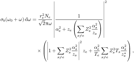
We start by describing the formalism developed by Cho et al. (Reference Cho, Sulzer and Kelley1998) and relevant equations that will be used in this work. The basic backscatter cross-section $\sigma _{b}$ equation is given by

where $\omega _{0}$ is the radar frequency and $\omega$
 is the Doppler frequency shift from the radar frequency; $V$
 is the radar volume, $r_{e}^{2}$
 is the classical electron radius, ${\rm \Delta} N_{e}$
 describes the electron density fluctuation spectrum and $k$
 is the Bragg wavenumber. The backscatter in the presence of charged dust can be described as (Cho et al. Reference Cho, Sulzer and Kelley1998)
where $T_{s}$ is the constituent temperature (the $s$
 constituents refer to ions and dust, positive or negative), $T_{e}$
 is the electron temperature and $N_{e}$
 is the electron number density. Here, we have included the charge number $Z_s^{2}$
 , where Cho et al. (Reference Cho, Sulzer and Kelley1998) have chosen to set this as $Z_s^{2} = 1$
 , which is often assumed valid for particles smaller than 10 nm. Note that everywhere the charge number is squared and thus the addition of dust does not depend on the sign of the charge except in the assumption of charge neutrality. The constant $\alpha _{s}$
 for each constituent $s$
 is given by

with $\lambda _{Ds}$ being the Debye length, $N_{s}$
 the number density of each component, $k_{b}$
 is the Boltzmann constant and $e$
 is the elementary charge. Then $z_{s}$
 is given by
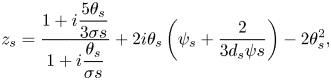
with $d_{s}$ as the viscosity constant (the value used is given in table 1) and $\psi _{s}$
 is the normalized constituent–neutral collision frequency, here given by

where $\nu _{sn}$ is the constituent–neutral collision frequency defined below for each constituent and $v_{s}$
 is the mean thermal velocity, which is given by

with $m_{s}$ as the component mass and the normalized frequency, $\theta _{s}$
 from (2.4), is given by

Now $\sigma _{s}$ (from (2.4)) is given by

with $m_{n}$ being the neutral mass and $c_{s}$
 the thermal conductivity constant (values used here is given in table 1). The collision frequency $v_{sn}$
 with neutrals in (2.5) depends on the particles in question. First, the electron collision frequency with the neutrals can be approximated as (Banks & Kockarts Reference Banks and Kockarts1973; Cho et al. Reference Cho, Sulzer and Kelley1998)

Collision frequency of other constituents with the neutrals can either be described by the so called polarization collision frequency or the hard-sphere collision frequency. For both positive and negative ions the former is preferred and further discussions on the validity of that choice can be found in Cho et al. (Reference Cho, Sulzer and Kelley1998). We assume a hard boundary of 0.5 nm for the size of the dust in relation to what collision frequency with the neutrals should be chosen and assume that this will not influence the spectrum in a large way. The polarization collision frequency is given by Banks & Kockarts (Reference Banks and Kockarts1973) and Cho et al. (Reference Cho, Sulzer and Kelley1998) as

where $M_{s}$ is the mass of the charged constituent in atomic mass units (amu), $F_{t}$
 is the fractional volume of the neutral gas present, $M_{nt}$
 is mass of each neutral component (in amu) and $\chi _{nt}$
 is the polarizability of those components. The values used in the calculations are given in table 1. The major neutral atmospheric constituents: molecular nitrogen and oxygen and atomic argon are taken into account. For the dust collisions with the neutrals both collision frequencies must be used. For the smaller dust sizes the polarization collision frequency is larger until the size reaches around 0.5 nm. Then the hard-sphere collision frequency starts to become larger and should be preferred. Thus for particles larger than 0.5 nm we use hard-sphere collisions with frequency (Schunk Reference Schunk1975; Cho et al. Reference Cho, Sulzer and Kelley1998)

where $r_n$ is the radius of the neutral particles. For neutral particles, we take an average radius of 0.15 nm (Cho et al. Reference Cho, Sulzer and Kelley1998). The collision frequencies for dust with neutrals thus can vary with dust size, mass density as well as the conditions of the neutral atmosphere. The influence these factors have on the spectrum are varied and we will examine them further in subsequent chapters.
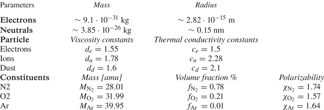
Table 1. Parameters and values used for calculations as inputs into equation (2.2). Values from Cho et al. (Reference Cho, Sulzer and Kelley1998). The constants given remain the same and are not changed for any of the calculations.
2.2. Incoherent scatter spectrum
To illustrate the parameters that we will discuss in the following sections, we start by presenting in figure 1 the spectrum in the presence of positively charged dust, because this changes most clearly in comparison with the spectrum without dust. The solid line describes the typical D-region spectrum, the dashed line describes the spectrum with an added positive dust component. The influence of the dust can be seen in the central part of the spectrum which is displayed in the figure. It is often denoted as the ion line and it contains the vast majority of the back-scattered power. The inclusion of dust causes the amplitude of the spectrum to increase and the corresponding width of the spectrum narrows as is illustrated in panel (a) of figure 1 showing the back-scattered power as a function of the frequency shift (equation (2.2)). Here and in subsequent discussion we refer to the width as the half-width-half-maximum (HWHM) value of the spectrum.
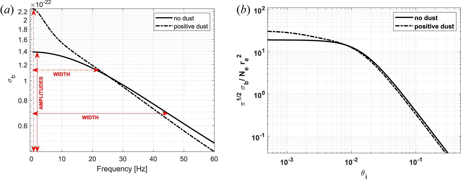
Figure 1. The central part of the incoherent scatter spectrum, ion line, calculated for conditions without dust and for different dust components is shown on the left; and the amplitude and width are indicated for both spectra. The figure on the right shows the corresponding normalized spectra; parameters used for the calculations are described in the text.
Following the presentation of calculated spectra by Cho et al. (Reference Cho, Sulzer and Kelley1998) and other authors, we show in figure 1(b) the same spectra with respect to the normalized frequencies (2.7). Note here the logarithmic scale and broader range of frequency. The spectra shown in the figure are calculated for the EISCAT VHF frequency of 224 MHz; this frequency is used throughout the paper. Other parameters used in these calculations are a constant electron density of 5000 cm$^{-3}$ for each individual spectrum calculation while the amount of dust present was set to 1000 cm$^{-3}$
 and the positive ion density thus set to 4000 cm$^{-3}$
 to keep charge neutrality. If not mentioned otherwise, we use for the calculation singly charged dust, ion mass of 31 amu, neutral density of $5 \times 10^{14}$
 cm$^{-3}$
 and electron density values for 85–90 km height.
As can be seen in the figures, the presence of charged dust narrows the width of the spectrum and increases the central amplitude. This occurs independent from charge polarity but is most prominent for only positive dust particles and less so in the presence of negative and positive dust or of only negative dust. We choose in this paper to focus on the spectrum and the corresponding frequency as is seen in part (a). What we are interested in further is to examine the different parameters of the background atmosphere as well as the dust properties that might be present and how these influence both the spectrum amplitude and the width. And thus in the following sections we show for various cases the spectrum amplitude change on one side and the spectrum width on the other.
3. Dusty plasma conditions and influence of dust parameters
3.1. Dusty plasma conditions
The incoherent scatter from the D-region that we examine here is an example of dusty plasma, where the presence of charged dust particles changes the properties of the plasma. Goertz (Reference Goertz1989) defines dusty plasma as an ensemble of dust particles in a plasma consisting of electrons, ions and neutrals. The dust charging leads to interactions with the surrounding plasma and charged dust particles are included through the charge neutrality condition describing the plasma. The charged dust particles are further influenced by electromagnetic forces and can be described as an additional ion component with a different charge to mass ratio. In a more narrow sense, dusty plasma describes conditions when the charged dust particles participate in the screening process rather than acting as isolated particles. For dusty plasma according to this latter definition (Mendis & Rosenberg Reference Mendis and Rosenberg1994; Verheest Reference Verheest1996), the dust grain size, $r_d$ , inter-particle distance $a$
 and plasma Debye length, $\lambda$
 are such that $r_d \ll a < \lambda$
 . This relation holds for the conditions in the D-region ionosphere that we consider here (figures are shown in Appendix A).
3.2. Dust size distributions
The model can easily accommodate any size distribution of dust when calculating the spectrum. Let us consider three power law distributions where the number density is inversely proportional to the radius raised to the power of 0.5, 1.5 and 2.5; the number densities are constrained to 2000 cm$^{-3}$ (see figure 18 in Appendix A). We use geometric size bins with the volume 1.6 times the previous size because this description is also used in dust transport models (Megner et al. Reference Megner, Rapp and Gumbel2006). Figure 2 compares the spectra calculated for the size distributions with those calculated with an average dust size. One can see that assuming an average dust size, as was done by other authors, provides a good result for steep size distributions (figure 2c) but fails to describe the spectra for a flatter dust size distribution. Thus obtaining an average size from spectra that are strongly influenced by the larger particles would overestimate the derived average size by a large amount.
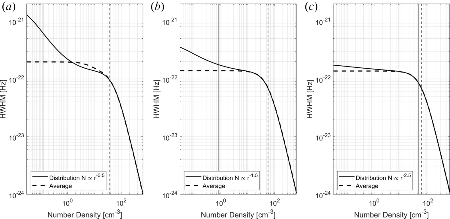
Figure 2. Spectrum shown for size distributions with different power laws given in figure 18 in Appendix A. Shown here with the spectrum calculated for the average size for each respective distribution. The number density of electrons is 5000 cm$^{-3}$ and total number density for dust is chosen as 2000 cm$^{-3}$
 of negative particles. The vertical lines show the spectral width of each respective spectral line.
3.3. Dust charge state
To investigate the influence of dust charge, we display the width of calculated spectra in figure 3. All cases shown are for negative dust particles (for positive particles see figure 19 in Appendix A). Figure 3(a) shows that the width of the spectra for different dust sizes and charge states 1 and 2 because the majority of dust in the D-region probably has small charges states (Baumann et al. Reference Baumann, Rapp, Anttila, Kero and Verronen2015). One can see that the width of the spectra does not vary a lot with dust density for small particles, while the spectral width changes with density for the larger dust particles. This change depends in addition on the charge state. In 3(b) we show how the width changes for a 10 nm particle with several different charge numbers. For small negative charge, the spectrum is broad for small dust densities and then narrows. For charge states 5 and higher, the spectra are in general very narrow and the width increases with dust density. We point out that the charge assumptions here are made for illustration and a discussion of charging models is beyond the scope of this work.
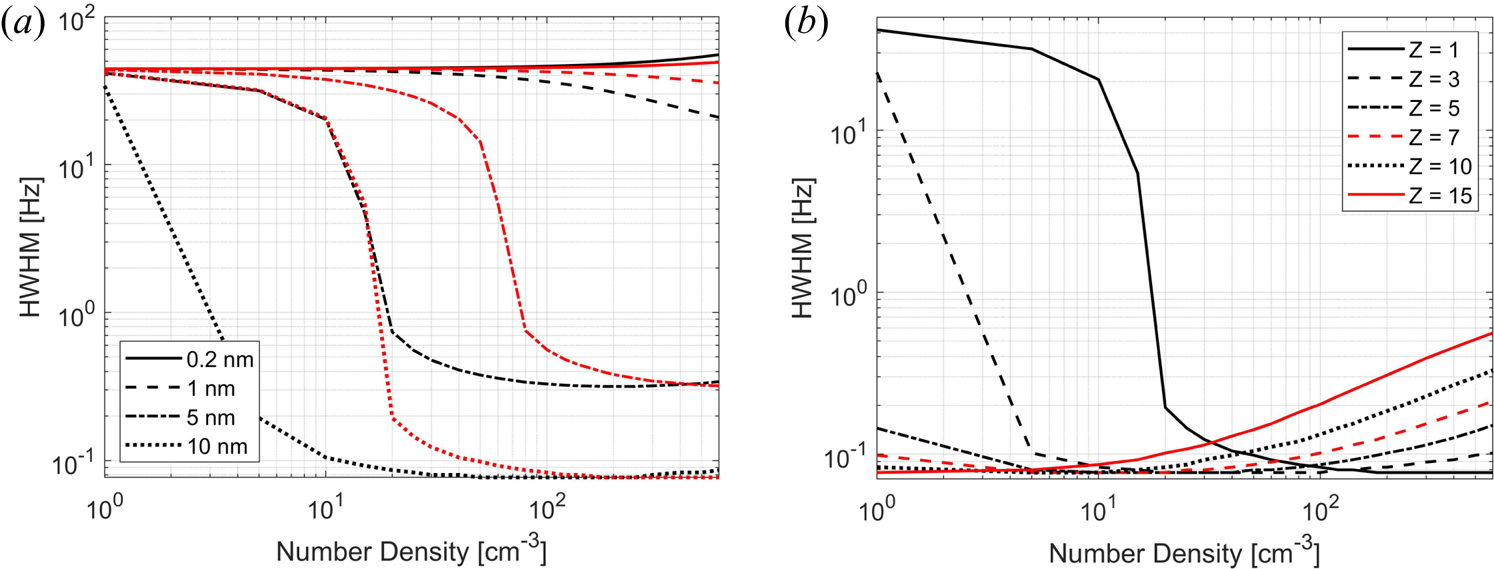
Figure 3. Spectral width (Hz) shown as a function of number density (cm$^{-3}$ ) for negative dust particles. In (a) several dust radii are shown for two different charge numbers Z where the red lines show $Z = 1$
 and black lines show $Z = 2$
 . In (b) we show the spectral width for 10 nm particles for several charge numbers Z; (a) $Z_d = 1$
 and 2 for $r_d = 0.2$
 , 1, 5, 7 and 10 nm and (b) $Z_d = 1$
 , 3, 5, 7, 10 and 15 for $r_d = 10$
 nm.
nm.
3.4. Model limitations
We use this model approach to investigate the influence of dust at 60–100 km altitude on the incoherent scatter. The model applies to a plasma that is collision dominated and weakly ionized (Cho et al. Reference Cho, Sulzer and Kelley1998). The frequencies of collisions of the charged particles with neutrals are high and any magnetic field effects as well as collisions between the charged particles can be neglected. Because of the high neutral density and predominance of collisions with neutrals, the temperatures of the different components can be considered equal. If the dust density in this region is large enough, it can influence the surrounding plasma and affect the spectra measured with radar.
4. Variation of the spectrum with ionospheric and dust parameters
We now investigate how the scatter spectrum depends on the dust properties and atmospheric conditions. Our calculations are made for mesospheric conditions at the location of the EISCAT VHF radar in Northern Norway (69.58$^{\circ }$ N and 19.23$^{\circ }$
 E); they also apply for the new EISCAT$\_$
 3D system, because both locations are less than 50 km apart. The MSPs are thought to reside at altitudes ranging in the D-region so we consider altitudes from 60 to 100 km for which we need to assume typical values for electron density, ion density and mean ion mass, neutral density and neutral temperature and their variation with height and in a course of a year.
We assume the electron density given in the International Reference Ionosphere (IRI2012) model (Bilitza Reference Bilitza2001) and the neutral density and temperature obtained from the MSISE model (NRLMSISE-00 Picone et al. Reference Picone, Hedin, Drob and Aikin2002). For all calculations, the temperature of each constituent is assumed equal to the neutral temperature, which is a good approximation because the number densities of neutrals are high and therefore also their collision rates with the other constitutes. In the following, we discuss how different parameters influence the spectrum.
4.1. Electron background conditions
The number of electrons present at the altitudes in question is an important parameter because it determines the strength of the signal and signal to noise ratio (SNR) and hence accuracy and the quality of the measurements. To resolve plasma parameters, small SNRs require a longer integration time, which on the other hand, is limited by the variation of the ionosphere with time. To find typical values, we consider the electron density from the IRI model (Bilitza Reference Bilitza2001) at noon (UTC) for each day of the year of 2019, shown in figure 4 at altitudes 65 to 100 km. UTC time was chosen due to variation in local time between summer and winter and noon UTC time is quite close to the maximum background electron density values during the day. The figure includes a few contour lines describing equal electron densities. One can see that for most of the days, the electron density below 85 km, is less than $10^{9} \ \textrm {m}^{-3}$ or $1000 \ \textrm {cm}^{-3}$
 , which is a typical limit for studies with the EISCAT VHF. The year 2019 for which we selected the parameters is close to the solar minimum, so that we here consider the more challenging conditions of small electron content in the D-region. It is important to note that chances to measure spectra differ during disturbed conditions that occur for example during high solar activity. During certain times, the number of free electrons can increase by several orders of magnitude (Turunen Reference Turunen1993; Schlegel Reference Schlegel1995) so that radar signals can be obtained from heights as low as 60–70 km; as for instance, one study of the D-region spectrum mentioned above covered heights of 70-92 km (Hansen et al. Reference Hansen, Hoppe, Turunen and Pollari1991).
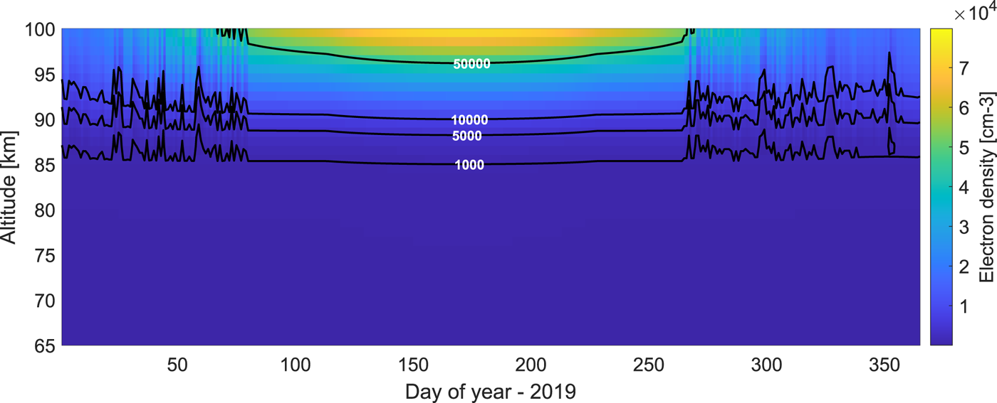
Figure 4. The electron density (${\rm cm}^{-3}$ ) above EISCAT location at noon (UTC) obtained from the IRI model (Bilitza Reference Bilitza2001). The colour scale gives electron number densities, lines of constant number densities are superimposed with lowest line describing EISCAT VHF approximate detection limit.
4.2. Temperature and neutral density
The temperature and the density of the neutrals in the D-region vary considerably throughout a year and with altitude and their influence on the spectrum is significant. The global atmospheric circulation causes an up-welling of air at high latitudes during summer and downward motion during winter in the mesosphere. As a result the densities below 90 km are higher in summer and diminished in winter; and the motion is associated with low temperatures in summer and warmer temperatures in winter. The temperature variations at altitudes 60–100 km over one year are displayed in figure 5(a). These data are from the IRI2012 model (Bilitza Reference Bilitza2001) at noon UTC for the year 2019 at the EISCAT VHF location. One can see a cold minimum during the summer months reaching down to 140 K and the warmer winter months with temperatures exceeding 200 K.
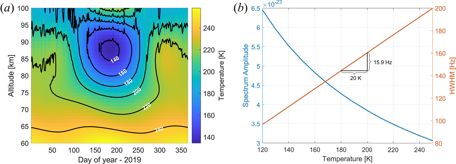
Figure 5. Temperature from the IRI model (Bilitza Reference Bilitza2001) for EISCAT location at noon (UTC) and year 2019 on the left and corresponding variation of the spectrum at 85 km altitude shown for the amplitude (blue line) and width (orange line) on the right.
The variation of the incoherent scatter spectrum with these temperatures can be seen in figure 5(b), which gives the corresponding variation of the spectral amplitude and width. One can see that the spectral amplitude increases with decreasing temperature while the width of the spectrum decreases. Increasing the temperature by for example 20$^{\circ }$ K reduces the spectral width by approximately 16 Hz, which also shows how temperature estimates influence the interpretation of the results.
Figure 6(a) shows the neutral density at 60–100 km altitude and noon UTC from the NRLMSISE-00 model (Picone et al. Reference Picone, Hedin, Drob and Aikin2002) during the year 2019. As can be seen, the density strongly varies from winter to summer, especially for the lower altitudes by almost a factor of 10 (not the log scale). An exception is the highest considered altitudes (above 95 km ca.) where the density is lower during the summer months compared with spring/autumn and a bit higher during the main winter months. Figure 6(b) shows the variation of the calculated spectrum for those conditions. The spectral amplitude increases with increasing neutral density. The spectral width initially increases with increasing neutral density and then decreases. The increase in the width is only for very low neutral density at the limit of our model calculations for summer conditions. For the winter conditions the spectrum only narrows for increasing altitude and decreasing neutral density.
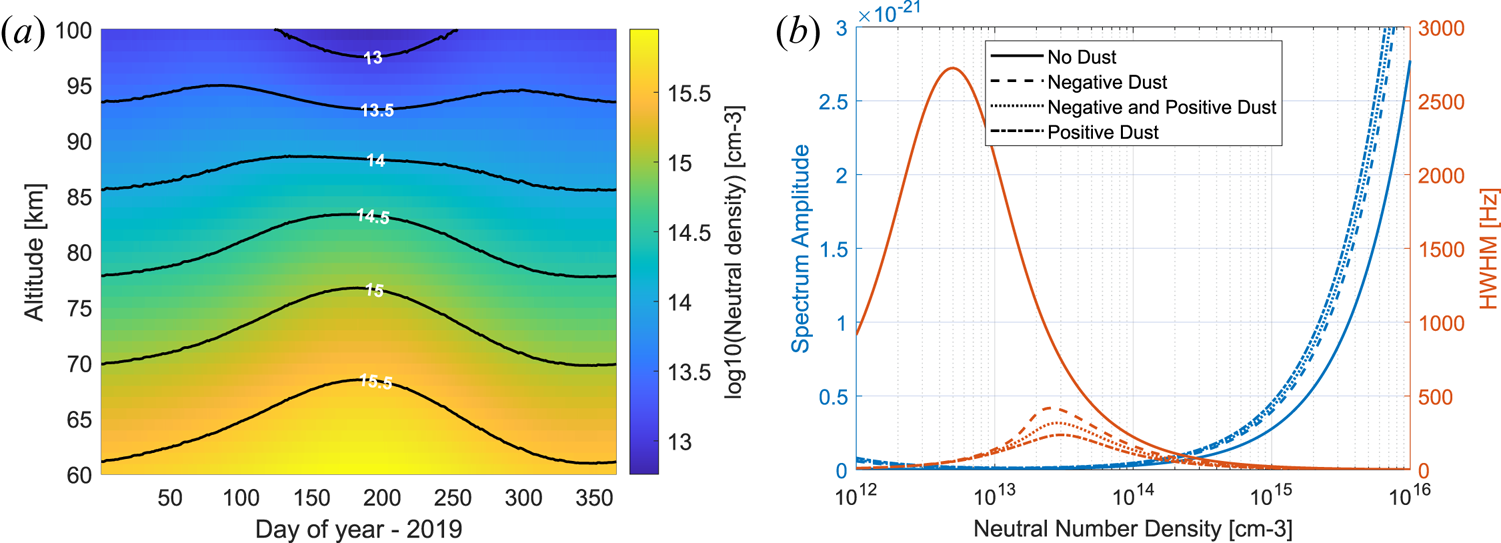
Figure 6. Neutral density from the NRLMISE-00 model for EISCAT location at noon (UTC) and year 2019 on the left and corresponding variation of the spectrum at 85 km shown with the spectral amplitudes (blue lines) and widths (orange lines) on the right calculated without dust and including different charged dust components as explained in the text.
4.3. Positive and negative ions
The composition of ions, both positive and negative, is more complicated in the mesosphere. This is especially true for the altitudes below around 80 km where negative ions start to appear. The inclusion of negative ions adds another complication to the derivation of the spectrum. For one, the ions are negatively charged due to attachments to electrons causing a depletion in the electron density, an important factor to have in order to detect strong enough signals from radars. And secondly, the negative ions cause a widening of the spectrum thus for spectrum calculations below 80 km the dust influence would seem diminished due to negative ion presence. Thus, investigating the spectrum below 80 km, is challenging both in terms of the observations as well as with regard to interpretation of the results.
For comparison, the main ion components at 80–100 km are O2+ and NO+ (with some variations during season). Since their masses are 30 and 32 amu respectively and their electron recombination rates are also similar, the variation in the ions mass is not so significant at these altitudes (see, e.g. Strelnikova et al. Reference Strelnikova, Rapp, Raizada and Sulzer2007; Friedrich et al. Reference Friedrich, Rapp, Plane and Torkar2011). While the presence of large positive ions, for example water clusters, would cause the mean value of the positive ion mass to increase and influence the spectrum.
Figure 7(a) shows the change in the amplitude of the spectrum for dust radii ranging from 0.2 to 10 nm and ion masses from 20 to 100 amu. One can see that for sizes of dust up to around 5 nm the ion size does not influence the resulting spectrum but for larger sizes of dust the spectrum becomes higher for the larger ion sizes (this is only including positive ions). In figure 7(b) the changes in spectral width are shown for dust sizes 0.2 to 5 nm and for the same variation in the ion mass. Here, we can see that for small ion mass the width is broader than for the largest sizes by approximately 15 Hz thus the largest ion sizes would cause a narrowing in the spectrum compared with the smallest. And since the main ion mass above 80 km is considered to lie in the 31 amu range we can see that at lower altitudes where the ion mass might be larger since the composition is more complex that the spectrum might be more narrow and interfere with the narrowing caused by the dust particles. This is, however, mostly true for the smallest particles. For the largest dust particles the width of the spectrum is less variable. In summary, we note that the change in molecular compositions and resulting mean ion mass influences the spectrum, however, to a smaller extent than the temperature does.
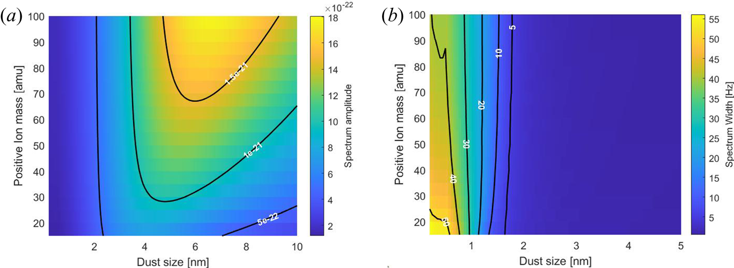
Figure 7. The variation of spectral amplitude (a) and spectral width (b) for different ion masses and dust radii.
4.4. Dust conditions
MSPs are thought to reside at altitudes around 60–100 km, with larger and fewer particles at lower altitudes and more abundant and smaller particles higher up. There is a strong indication that a fraction of the dust is electrically charged, and this portion of the dust is the one that theoretically can be detected with radar backscatter. The most important consideration in detecting the dust is the number of free electrons, too low density and the signal detected by the radar will not exceed the noise level. Too high electron content compared with the dust density and the dust will ‘disappear’ and thus not be detected. For the current EISCAT radar a number density of $1e9\ \textrm {m}^{-3}$ would be the absolute minimum for a good enough signal. Now for the dust density, that too needs to be in adequate numbers to be detected. Which we will examine here in more detail.
In order to investigate the distribution of MSPs in the atmosphere several authors have used atmospheric modelling. The earlier models mainly made one-dimensional (1-D) model calculations but thus disregarded the atmospheric circulation (Hunten et al. Reference Hunten, Turco and Toon1980; Megner et al. Reference Megner, Rapp and Gumbel2006). The dust distributions on a global scale, were studied in 2-D models that include the atmospheric circulation and some particle micro-physics. The results show that dust distributions are different in the equatorial regions and at the high latitudes (Bardeen et al. Reference Bardeen, Toon, Jensen, Marsh and Harvey2008; Megner et al. Reference Megner, Siskind, Rapp and Gumbel2008).
These differences in the distribution result from the influence of the global atmospheric circulation and the polar vortex at high latitudes which includes the EISCAT location considered here. The absolute number densities differ between different models, but are in a similar range as those obtained with the 1-D model, i.e. of the order of 1000 particles cm$^{-3}$ between mesopause and middle stratosphere (Hunten et al. Reference Hunten, Turco and Toon1980). For the discussion here, we choose the number density model with largest variation between winter and summer conditions which we take from Bardeen et al. (Reference Bardeen, Toon, Jensen, Marsh and Harvey2008).
4.4.1. Dust size, number density and bulk density
The spectrum varies greatly with dust size and different combinations of dust sizes will influence in a different way. In figure 8(a) the amplitude of the spectrum is shown for both positive and negative dust particles with radii from between 0.2 and 10 nm. The number density for the positive dust and the negative dust was kept the same, at 500 cm$^{-3}$ , while the electron and ion densities were varied to keep charge neutrality. For the negative dust the electron density was 5000 cm$^{-3}$
 and the positive ion density was at 5500 cm$^{-3}$
 . For the positive dust the number densities for the electrons was the same and for the positive ions the number density was at 4500 cm$^{-3}$
 .
.
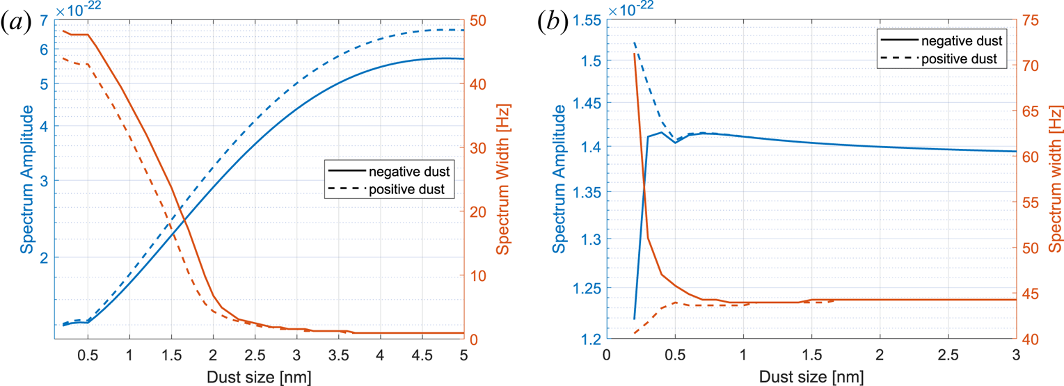
Figure 8. The spectral amplitude (blue) and spectral width (red) for positive (dashed lines) and negative (solid lines) dust particles with varying dust sizes shown in (a). Both negative and positive dust have number density of 500 cm$^{-3}$ in respective cases. In (b) the amplitude and width is shown for varying dust sizes but the number density is kept such that the total mass for each particle size is the same. The number density used for each dust size is shown in figure 21 in Appendix B.
The figure indicates that the presence of positive dust has a larger influence on the spectrum than negative dust; for both the amplitude and the width of the spectrum. This results from both the charge neutrality condition we keep, making the positive ion density lower by 1000 cm$^{-3}$ compared with the negative dust case as well as the fact that positive dust particles always cause a narrowing of the spectrum as while the negative dust causes a broadening for dust particles smaller than approximately 1 nm. This can be seen in figure 8(b). Here, the dust number density is varied for each size of dust so that the total mass of dust used in the calculations is kept constant. Thus for 3 nm dust size the number density is 1 cm$^{-3}$
 and this increases for decreasing size. The number densities used are given in figure 21 in Appendix B. Here, we can clearly see that for equal mass the width of the respective spectrum is narrowing for the positive dust while it is broadening for small dust sizes and narrowing for increased size. In figure 20 in Appendix B we give a 3-D figure for the variation of the spectrum with different dust size and densities.
As was previously mentioned the dust bulk density is unknown but has been suggested to be approximately 2–3 g cm$^{-3}$ by several authors (Hunten et al. Reference Hunten, Turco and Toon1980; Megner et al. Reference Megner, Rapp and Gumbel2006; Bardeen et al. Reference Bardeen, Toon, Jensen, Marsh and Harvey2008) and these are typical values for silicate particles. We choose for the calculations 3 g cm$^{-3}$
 but the results are not so different for 2 g cm$^{-3}$
 as we will see here. A larger variation in the density could occur if the particles have an irregular porous structure. The spectrum equation (2.2) is dependent on the mass of the particles and to calculate this we need to assume spherical particles of a certain mass density, the particles are definitely not spherical but we assume the mass difference using this assumption is negligible.
Comparison of spectrum calculations for bulk density 1 and 9 g cm$^{-3}$ (1000 and 9000 kg m$^{-3}$
 ) for the dust particles is shown in figure 9 for both negative dust in (a) and positive dust (b), showing that, for both the amplitude and the width of the spectrum, the variation is very small for dust larger than 0.5 nm. The largest difference is for particles smaller than 0.5 nm, however, the difference is at most a few Hz for the width and thus should not be influential in deriving the width from radar measurements except for cases with a very large number of small dust particles since the difference is also dependent on the number density of dust.
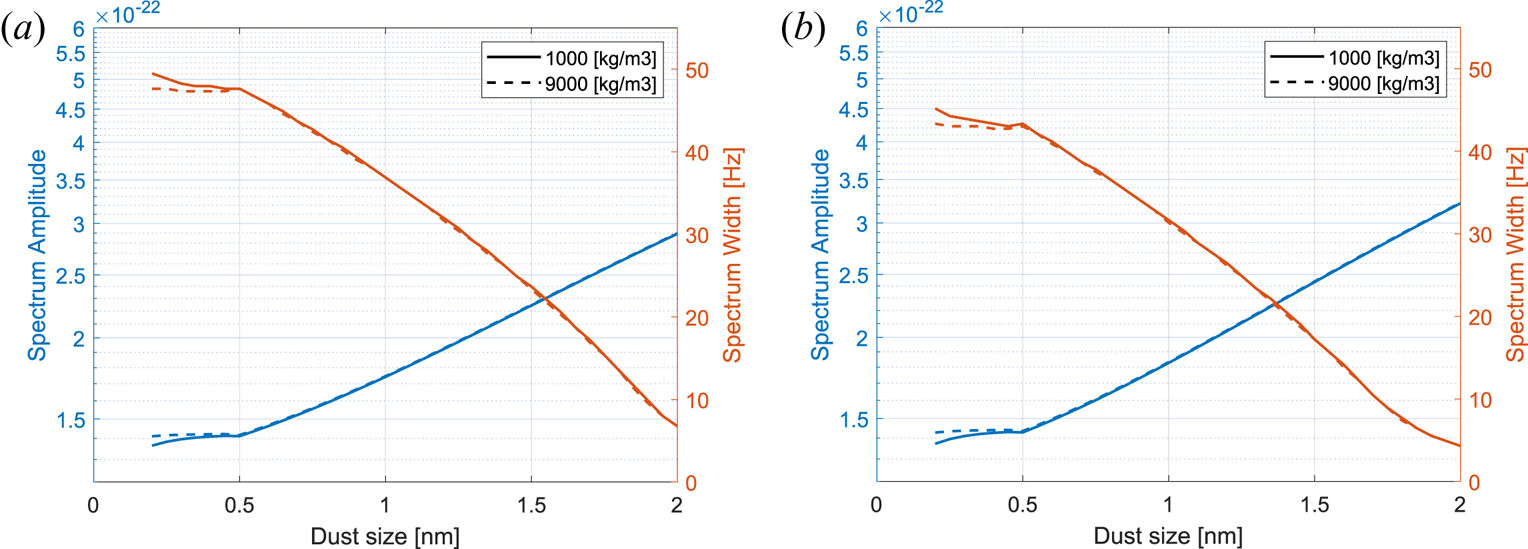
Figure 9. Variation in the spectrum amplitude and width for two different bulk densities of dust, 1000 and 9000 kg m$^{-3}$ respectively. Dust number density kept at 500 cm$^{-3}$
 and electron density at 5000 cm$^{-3}$
 while the positive ion density was varied to keep charge neutrality. (a) Negative dust and (b) positive dust.
4.4.2. Amount of charged dust and charge balance
The amount of dust that is charged is a subject of debate and largely depends on the charging model assumed. The results either conclude on approximately 6 % of the particles being charged or close to 100 % (Rapp et al. Reference Rapp, Strelnikova and Gumbel2007; Baumann et al. Reference Baumann, Rapp, Anttila, Kero and Verronen2015; Plane, Feng & Dawkins Reference Plane, Feng and Dawkins2015). This, however, is highly unlikely since allowing all the dust to become charged would in some cases remove all the free electrons from the D-region (Baumann et al. Reference Baumann, Rapp, Anttila, Kero and Verronen2015), which is especially true for the higher altitudes where the smallest dust sizes are assumed to be most abundant and could equal the number of free electrons present (Megner et al. Reference Megner, Rapp and Gumbel2006, Reference Megner, Siskind, Rapp and Gumbel2008).
Now the positive and negatively charged dusts influence the spectrum in different ways. This is due to the charge neutrality requirement we impose on the calculations, so that increasing the amount of positive dust would either increase the number of electrons or decrease the number of positive ions for example. In figure 10, the spectrum amplitude and width are shown for varying number density of negative and positive dust particles. So the electron density is kept constant and the dust particles are varied from 0 to 2000 particles cm$^{-3}$ for negative dust and from 2000 to 0 cm$^{-3}$
 for the positive dust, so that the total number density of charged dust is kept constant at 2000 cm$^{-3}$
 while the ratio of number of negative particles to positive particles is varied.
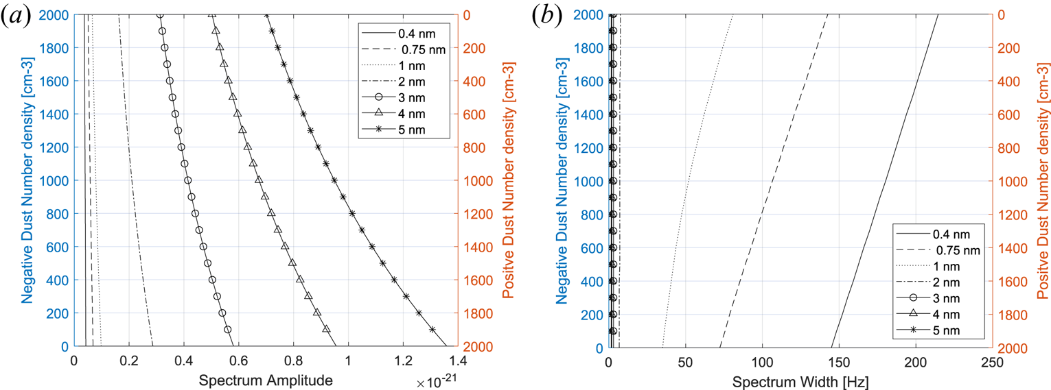
Figure 10. Spectral amplitudes and widths for selected cases of dust sizes: density of negative and positive dust particles is varied from 0 to 2000 cm$^{-3}$ and 2000 to 0 cm$^{-3}$
 , respectively. (a) Spectral amplitude and (b) spectral width.
One can see a stronger influence of the positive dust particles on the spectrum compared with the negative dust particles. The larger dust more influences the amplitude while the smaller dust particles influence the width and cause a narrowing of the spectrum. The narrowing of the spectrum could be more easily noted in the spectrum, because most of the other parameters broaden it.
We base our considerations of the influence of different number densities of charged dust on results obtained by Baumann et al. (Reference Baumann, Rapp, Anttila, Kero and Verronen2015) who combined an ionospheric chemistry model (Sodankylä Ion-Neutral Chemistry (SIC) model) and the MSP distribution modelled by Megner et al. (Reference Megner, Rapp and Gumbel2006) to study the influence of MSPs on the D-region charge balance. They found large differences in the charging conditions between positive and negative dust particles and strong diurnal variations. The negative particles showed a rather large number density during night at approximately 80–100 km due to effective electron attachment. The positive dust particles were most abundant during daytime at low altitude (55–75 km) and they were less abundant at night when they were located at higher altitude (up to 90 km) (see figure 22). This distribution poses several problems.
First, the negative dust particles mainly occur during night when electron densities are already low. Secondly, they form via electron attachment which further reduces the electron density. Figure 4 displays the noon variation of electrons from a solar minimum year and the electron density could be even further depleted in the presence of dust. From this we conclude that observational studies during the night are difficult, because the electron densities are low and therefore the SNR of observed spectra would not be optimal. As discussed above, positive dust particles would reduce the width of the spectrum to a larger degree than negative particles which could better be distinguished from the influences of other parameters. The conditions leading to positive charging of dust are, however, according to Baumann et al. (Reference Baumann, Rapp, Anttila, Kero and Verronen2015) best during the day at very low altitudes. The dust particles tend to be larger at low altitudes, making the detection even more promising, but the electron density is very low and even during the day often below the detection limit. The number of positively and negatively charged MSPs increases with an increased number of free electrons (Baumann et al. Reference Baumann, Rapp, Anttila, Kero and Verronen2015) caused, for example, by incoming photons or precipitating particles. Thus, a disturbed ionosphere with a high number density of electrons during daytime at low altitudes would be optimal.
5. Variations of the spectrum during the day and during the year
To investigate in detail observation conditions above the EISCAT site, we first carry out a case study regarding variation within 24 hours and then simulate spectra for ionospheric parameters varying over a year.
5.1. Case study – September conditions
The dust size and density distributions in the mesosphere are determined by transport and collisional growth in the neutral atmosphere (e.g. Hunten et al. Reference Hunten, Turco and Toon1980; Megner et al. Reference Megner, Rapp and Gumbel2006; Bardeen et al. Reference Bardeen, Toon, Jensen, Marsh and Harvey2008). The number of charged particles is determined by sunlight and ionospheric conditions,including ion chemistry reactions as simulated in a model by Baumann et al. (Reference Baumann, Rapp, Anttila, Kero and Verronen2015), which includes the dust distribution by Megner et al. (Reference Megner, Rapp and Gumbel2006).
We take the combined results for these two models as input to simulate the incoherent scatter spectrum. For comparison, we also simulate the spectrum in the absence of dust, assuming the parameters from the same model calculations done by Baumann et al. (Reference Baumann, Rapp, Anttila, Kero and Verronen2015). For the background parameters we use the NRLMISE-00 atmospheric model (Picone et al. Reference Picone, Hedin, Drob and Aikin2002) for the temperature and neutral density for the same time period as the data from Baumann et al. (Reference Baumann, Rapp, Anttila, Kero and Verronen2015), 24 h data for 7–8 of September 2010.
The calculated spectrum amplitude and width during these 24 hours are presented in figure 11 using negative and positive dust densities (shown in figure 22 in Appendix B). The dust particles were mostly negatively charged during the night and at high altitudes and mostly positively charged at low altitudes during the day; some positively charged dust is also found at higher altitude during night (figure 22). We calculated the spectra for these dust parameters and compared the results with those obtained without dust.
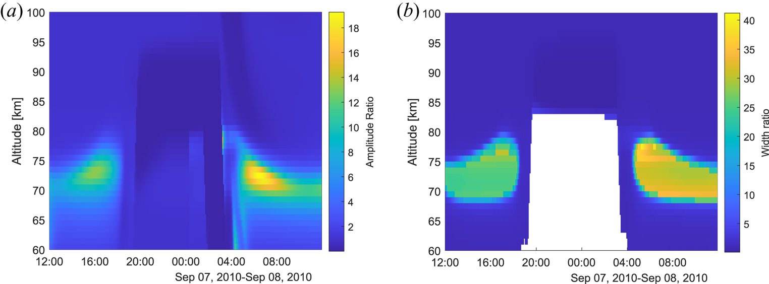
Figure 11. Spectrum amplitude ratio for dust to the no dust case shown in (a) and ratio of the width in (b) for no dust to the dust case; using values from noon to midnight 7–8 September 2010. White area depicts times and altitudes when the electron density is much lower than the dust density.
Figure 11(a) displays the amplitudes relative to amplitude without dust and in (b) the spectrum width for the no dust case is shown relative to the dust case. The strongest influence on the amplitude and on the width can be seen at lower altitudes, mainly during daytime. Here, the width seems to narrow much more for the dust case compared with the no dust case, i.e. up to approximately 40 times. Thus conditions to detect charged dust in this particular case would be best during the day and at altitudes of approximately 70–80 km. Looking at the ratio of positive dust to positive ions given in figure 24(b) there are similarities in the altitude range and time for when the amplitude and width are very influenced by the charged dust.
Note that the conditions below 80 km at night are not included in figure 11(b). This is because the electron density is very low, up to 300 times lower than the negative dust density, and hence the radar signal would be below the detection limit (see figure 24(a) in Appendix B). The charged dust would make the spectrum very narrow, however, so this time period could be considered for future radar observations if the electron density would be sufficiently enhanced above the radar detection limit.
According to Baumann et al. (Reference Baumann, Rapp, Anttila, Kero and Verronen2015) the presence of dust changes the D-region charge balance and the relative magnitude of each constituent present. Thus the data used here for the dust case and the case without the dust do not correspond in electron density or the amount of positive or negative ions. Thus, for radar observations it would be beneficial to run similar model calculations on the charge state to get the most accurate results on the relative narrowing of the spectrum.
5.2. Variation of the spectrum during the year
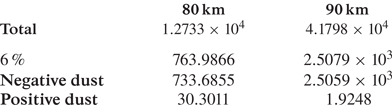
We now consider all parameters discussed above to investigate the variation of the spectrum during a year. To calculate the spectra, we used two different dust size distributions from Baumann et al. (Reference Baumann, Rapp, Anttila, Kero and Verronen2015): one at 80 km during the day (noon) where positive and large dust particles are more abundant and one at 90 km where small and negative particles are more abundant, the distributions are shown in figure 12. The total number densities of the dust are from Bardeen et al. (Reference Bardeen, Toon, Jensen, Marsh and Harvey2008) for average summer dust number densities which are smaller than their average winter values. We assume that 6 % of this total dust number density is charged with values used given in table 2. We then calculate the spectrum for the altitudes 80 km and 90 km using model assumptions for electron densities and relative ion composition from the IRI model (Bilitza Reference Bilitza2001) (figure 4) and the neutral density (figure 6) and temperature (figure 5) from the NRLMISE-00 model (Picone et al. Reference Picone, Hedin, Drob and Aikin2002).
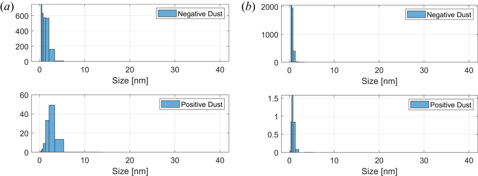
Figure 12. Size distributions of negative and positive dust particles, further explained in the text. (a) Dust number density in cm$^{-3}$ at 80 km and (b) dust number density in cm$^{-3}$
 at 90 km. The top panel shows negative dust and bottom panel shows positive dust.
Table 2. Number densities (in cm$^{-3}$ ) of dust used in calculations of figures 13, 14 and 15 in § 4.2 where we have used a total of 6 % of the total dust density as charged dust for both 80 km and 90 km. The total number densities are from Bardeen et al. (Reference Bardeen, Toon, Jensen, Marsh and Harvey2008), where we have used the average number densities for these altitudes for summer conditions (approximate). Number of negative dust vs. positive dust comes from the size distributions from Baumann et al. (Reference Baumann, Rapp, Anttila, Kero and Verronen2015) for 80 km and 90 km.
First, we present calculations for 90 km altitude in figure 13, showing the amplitude of the spectrum (panel a) and the width (panel b). We compare spectra with dust (red dotted line) and without dust (the solid blue line). The electron density here is of order 5000 cm$^{-3}$ or more for most of the year (cf. figure 4) and therefore exceeds the total dust number densities that we considered. One can see that the dust increases the width of the spectrum. This is caused by the small dust particles that are largely dominant in the assumed size distribution (see figure 8). The charge neutrality condition is also important here, and we keep the electron density as given from the IRI model (Bilitza Reference Bilitza2001) for the year 2019, while we vary the positive ions to keep the charge neutrality due to the increased negative dust particles.
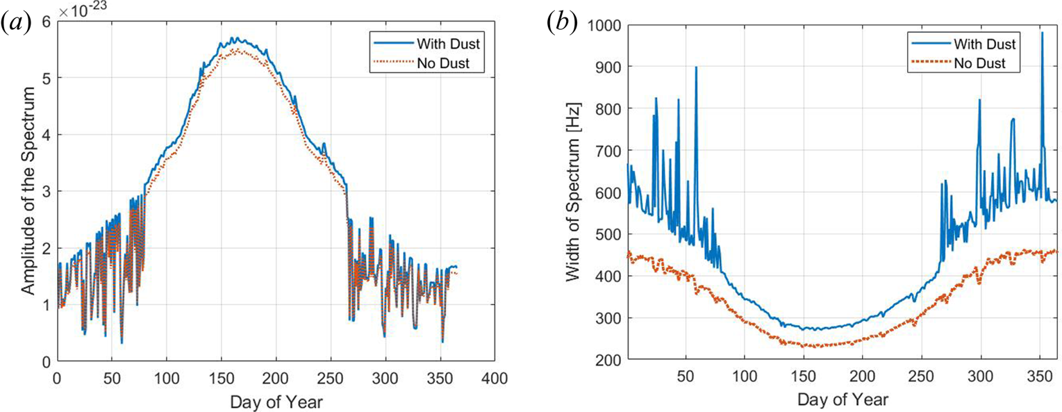
Figure 13. Amplitude and width for spectrum calculations for altitude of 90 km and a dust number density shown in figure 12(a). (a) Spectrum amplitude and (b) spectrum width.
Results for spectra at 80 km altitude are shown in figure 14. One can see that the amplitudes are much higher in the case when dust is included, while the spectral width is reduced. This is because the large dust particles included here lead to a more narrow spectral width, as mentioned above. This result, however, describes a case that because of low electron density cannot be observed, or at least not with the systems we are aware of. For the sake of investigating the spectra, we now assume an enhanced electron density ($\sim$ 90 km) for otherwise 80 km conditions.
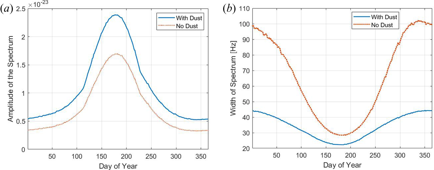
Figure 14. Amplitude and width for spectrum calculations for altitude of 80 km and a dust number density shown in figure 12(b). (a) Spectrum amplitude and (b) spectrum width.
In such a case, the amplitude difference between the dust and no dust cases is largest during the summer. The differences in the width of the spectra are most pronounced during the winter while the summer spectra do not much differ between the cases with and without dust where both spectral widths are quite narrow due to the cold mesospheric temperatures. The presence of charged dust in both cases narrows the spectra at 80 km and variations during the year are less pronounced than they are without dust. The spectral width is approximately 20 % narrower during the winter months, which corresponds well to the discrepancy found by Hansen et al. (Reference Hansen, Hoppe, Turunen and Pollari1991) for similar altitudes under enhanced electron density conditions.
Note that, during winter, the electron density in the IRI model (Bilitza Reference Bilitza2001) fluctuates from day to day and because of this all calculated parameters shown in the figures fluctuate during the winter months, i.e. roughly the first and the last 90 days of the year. The cyclic nature of the curves, easy to see in the red curve representing the no dust scenario, can mainly be attributed to the background variations. For example, the temperature being higher in the winter which produces a wider spectrum while a lower temperature narrows the spectrum; this is also the case for the temperature minimum of the summer mesosphere. The spectrum is also broader because of a typically higher neutral and electron density during summer, which is due to up-welling of air at the northern pole (polar vortex). We point out that investigations during summer at mid and high latitude can be further complicated by the formation of strong coherent radar echoes called polar mesospheric summer echoes (see e.g. Rapp & Lübken Reference Rapp and Lübken2004) The cold temperature in the mesosphere during the summer causes large ice particles to form in the altitude range 80–90 km, using dust as condensation nuclei. These can become charged and turbulence causes structures in these charged ice particle clouds that cause large electron density gradients and subsequently powerful coherent radar echoes. The presence of these coherent radar echoes would make it difficult to detect the much weaker incoherent radar signal.
6. Summary and conclusions
We investigate the incoherent scatter from the D-region ionosphere taking into account the influence of charged dust particles. The model is based on the previously used fluid description of a weakly ionized plasma and charged dust (Cho et al. Reference Cho, Sulzer and Kelley1998). In our calculations we include dust particles with a size distribution and, different from previous works, we include also different charge states of the dust. We show that the charge number has a strong influence on the spectra for large particle radii. However, based on present understanding of the dust charging in the ionosphere, we expect the dust particles to be typically singly or at best doubly charged; in this case the differences are not so strong for particles in the smaller size range, which are the dominant sizes in the D-region, excluding conditions favouring ice particle formation in the summer mesopause.
While the backscatter cross-section does not change with the charge polarity of the dust, we find that the spectra strongly differ between the positively and negatively charged dust particles. This is because they contribute in different ways to the charge balance. Positive dust particles are easier to detect because they are associated with a decrease in the ion component. The lack of ions narrows the spectrum so that the influence of the charged dust becomes more apparent.
We discuss the dusty plasma conditions and show that it is valid in the D-region ionosphere for all conditions we considered here. We find, however, that it is hard to derive information on charged dust from observed spectra for a number of reasons.
We consider the conditions at the EISCAT VHF radar with 224 MHz transmit frequency and find that the spectrum can narrow due to the presence of dust by up to 50 Hz (HWHM). The positive dust particles influence the spectrum more strongly than negative dust particles and we find high dust number density to be quite important. Models predict higher numbers of large positive dust particles during the day at lower altitudes as opposed to during the night (Baumann et al. Reference Baumann, Rapp, Anttila, Kero and Verronen2015).
Conditions are more favourable for dust detection during the winter compared with summer conditions, mainly because in the winter mesosphere we expect higher temperature, lower neutral density and higher dust number density (Megner et al. Reference Megner, Rapp and Gumbel2006). The electron density during observations needs to be high enough so that the SNR of the measurements is sufficient to analyse the spectra. This latter requirement is somewhat in contradiction to the best spectra being expected at low altitude. A target condition to search for dust signatures in the spectra is therefore during special ionospheric conditions when the electron content is large below 80 km. We will consider these results to choose the most suitable observational data and observation conditions in future work.
In summary we see that the spectra depend on a number of different parameters. It would therefore be helpful to derive some parameters independently from other observations along with any radar measurements in order to accurately determine the spectrum and distinguish the dust signatures from those of the other parameters.
Both the temperature and the density of the neutral atmosphere can influence the spectrum in various ways. Temperatures vary a lot throughout a year and also locally and with height; a 20 K temperature change can alter the width of the spectrum by almost 20 Hz. Independent temperature and neutral density observations can be made using LiDAR (Light Detection and Ranging, cf. Nozava et al. Reference Nozawa, Kawahara, Saito, Hall, Tsuda, Kawabata, Wada, Brekke, Takahashi, Fujiwara, Ogawa and Fujii2014). Additional electron density measurements can be made using ionosondes. In situ observations with rockets can provide independent information at a given time and location on the charge and size distributions of dust, on the neutral density and on the neutral temperature.
To carry out this study, we have developed a code to calculate the incoherent scatter spectrum, including a set of size bins for charged dust particles; different from and extended from previous codes, we include dust components with different charge numbers. The code is open access at the repository of UiT, Arctic University of Norway (see Appendix C).
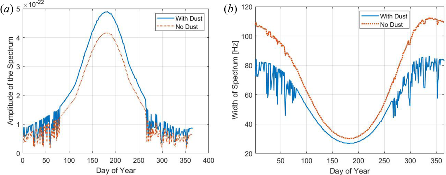
Figure 15. Amplitude and width for spectrum calculations for altitude of 80 km with electron number density from 90 km and a dust number density shown in figure 12(a). (a) Spectrum amplitude and (b) spectrum width.
Acknowledgements
We thank C. Baumann, DLR Neustrelitz for providing dust distribution data and for helpful discussions. The code that we developed is based on previous codes by Strelnikova (Reference Strelnikova2009) and Teiser (Reference Teiser2013). Thanks to A. Poggenpohl for good discussions and input to code changes. Simulation results have been provided by the Community Coordinated Modeling Center at Goddard Space Flight Center through their public Runs on Request system (http://ccmc.gsfc.nasa.gov). The IRI Model was developed by D. Bilitza at the NASA/Goddard Space Flight Center and the NRLMSISE-00 Model was developed by A.E. Hedin at the NASA/Goddard Space Flight Center. The data/code that support the findings of this study are openly available from UiT Open Research Data at https://doi.org/10.18710/GHZIIY.
Editor Edward Thomas, Jr. thanks the referees for their advice in evaluating this article.
Funding
This work was supported by the Research Council of Norway (grant number NFR 275503) and the publication charges for this article have been funded by a grant from the publication fund of UiT, The Arctic University of Norway.
Declaration of interest
The authors report no conflict of interest.
Appendix A. Dusty plasma conditions
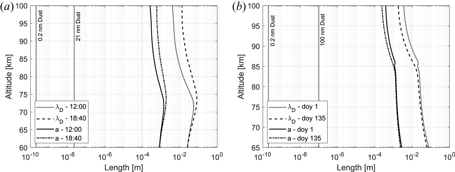
Figure 16. The figures show dust sizes, mean distance between plasma particles a and plasma Debye length $\lambda$ for conditions used in the case studies for September conditions in (a) and two days in 2019 (b). One can see that the relation $r_d \ll a < \lambda$
 is always valid. It would hold even for large particles up to 100 nm. We approximate $a \propto N_e^{-1/3}$
 .
.
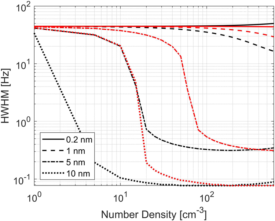
Figure 17. Spectral width (Hz) shown as a function of number density ($cm^{-3}$ ) for positive dust particles with two different charge numbers. Charge number $Z = 1$
 is shown in red and $Z = 2$
 is shown in black.
Appendix B. Supporting figures on D-region conditions
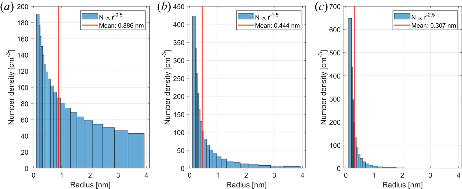
Figure 18. Dust size distributions with three different power laws, $r^{-0.5}$ , $r^{-1.5}$
 and $r^{-2.5}$
 , each with a total number density of 2000 cm$^{-3}$
 . The average size is marked in the histograms in red. We choose 20 size bins that are calculated from the initial size of 0.2 nm using a geometric distribution as the one used by Megner et al. (Reference Megner, Rapp and Gumbel2006).
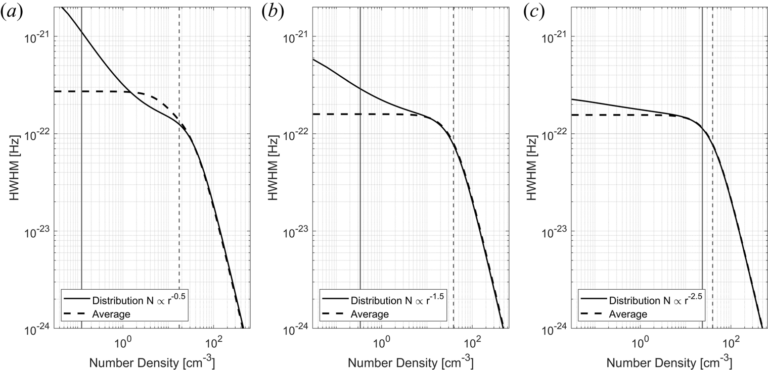
Figure 19. Spectrum shown for size distributions with different power laws given in figure 18. Shown here with the spectrum calculated for the average size for each respective distribution. The number density of electrons is 5000 cm$^{-3}$ and total number density for dust is chosen as 2000 cm$^{-3}$
 of positive particles.
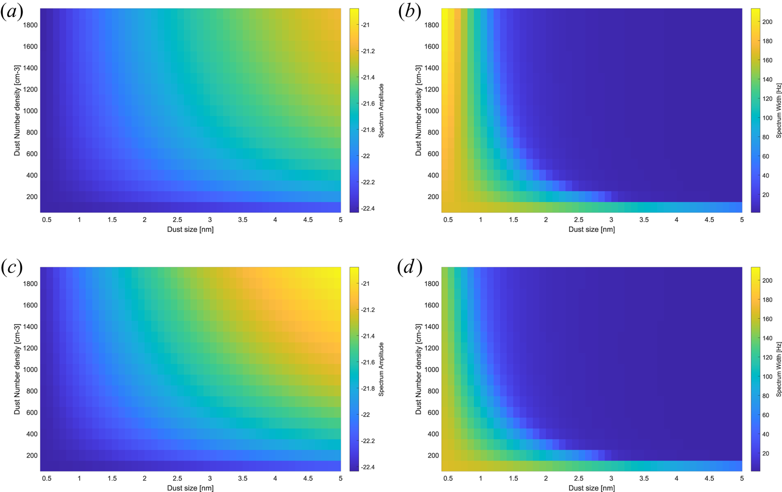
Figure 20. Spectral amplitudes and widths calculated for negative and positive dust particles, respectively, as a function of dust radius with radii ranging from 0.4 to 5 nm (horizontal axes) and as function of dust number densities from 50 to 2000 cm$^{-3}$ given on the vertical axes. (a) Negative dust – amplitude, (b) negative dust – width, (c) positive dust – amplitude and (d) positive dust –width.

Figure 21. Dust number density in cm$^{-3}$ used in figure 8.
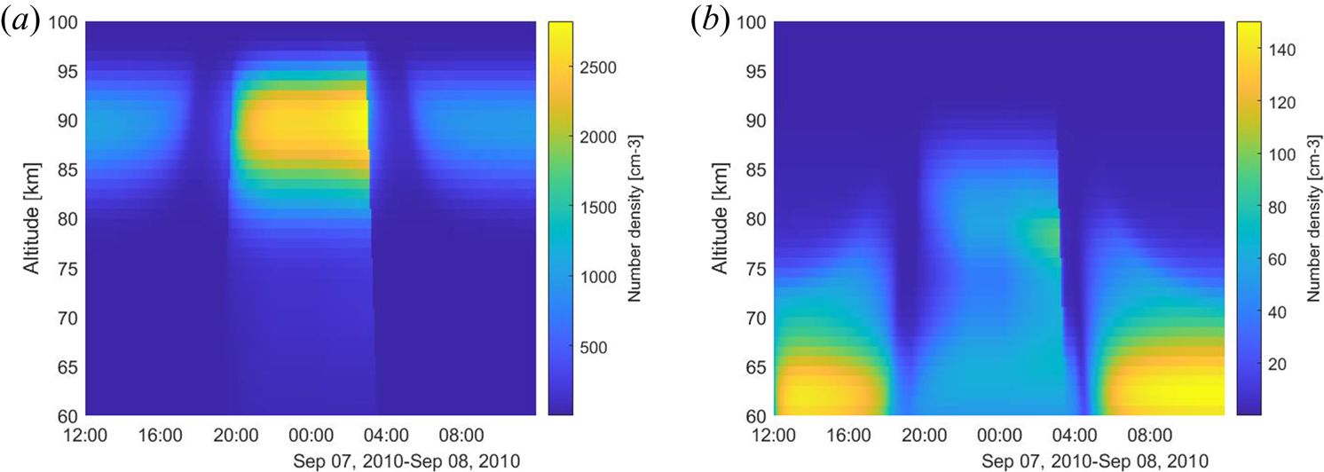
Figure 22. Number densities of charged dust for conditions from noon to midnight 7–8 September 2010; these are used for the model calculations presented in § 5.1 (from Baumann et al. (Reference Baumann, Rapp, Anttila, Kero and Verronen2015), courtesy of the author). (a) Negative dust density cm$^{-3}$ and (b) positive dust density cm$^{-3}$
 .
.

Figure 23. Spectrum width ratio calculated for the parameters used in the case study from § 5.1 where the smallest electron densities are included as well. Here, the ratio is the spectral width for the no dust case to the spectral width for included dust.
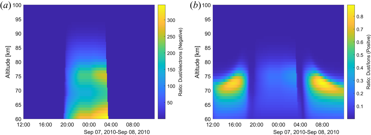
Figure 24. Ratio of the negative dust to electrons on the left and positive dust to positive ions on the right. Data from Megner et al. (Reference Megner, Rapp and Gumbel2006) and Baumann et al. (Reference Baumann, Rapp, Anttila, Kero and Verronen2015) used in § 5.1.
The spectrum varies with dust size but also the amount of dust for each size. Since we do not have an adequate amount of information on what size distributions we could expect at each time, we can get a closer look at how the spectrum varies for a certain dust size and with number densities. In figure 20 we show the amplitude and width of the spectrum for positive and negative dust and how each size varies with a respective number density. For negative dust, the amplitude and width in (a) and (b) are similar to the amplitude and width of the positive particles. The amplitude is higher for positive dust, especially for large sizes, and the width is broader for negative dust in the smaller size regime. Both positive and negative dust show a narrower spectrum for larger dust sizes. The negative particles also show that the widest spectrum happens for the smallest sizes and largest number densities. Both positive and negative particles show that, for vary small number densities, the spectrum is at its widest. This is interesting to note since for large dust sizes the number density will most likely always be very small and thus its contribution to the narrowing of the spectrum is large even for just a few particles.
Dust number density for different sizes is shown in figure 21 where the total mass has been assumed the same regardless of size and the particles assumed to be spherical and have bulk density of 3000 kg m$^{-3}$ and we choose the total mass to be the same as 1 particle of 3 nm size.
Number densities used in § 5.1 are shown in figure 22 with negative dust number densities on the left and positive dust number densities on the right. These data are from Baumann et al. (Reference Baumann, Rapp, Anttila, Kero and Verronen2015) and are courtesy of C. Baumann.
We include all the spectrum amplitudes, as well as those that are very low and have almost no electron density present, in figure 23, where we can see large narrowing in the spectrum during night for altitudes 70 to 80 km. This case, however, has electron densities almost 300 times smaller than the negative number density, as can be seen in figure 24(a), where we show the ratio of the negative dust particles to the electron density. The ratio of positive dust to positive ions is shown in (b) with the areas of largest difference corresponding well with areas of largest narrowing of the spectrum width shown in § 5.1.
Appendix C. Code
We have developed a code to calculate the incoherent scatter spectrum including a set of size bins for charged dust particles. The code is written in MATLAB. It was developed based on previous codes by Strelnikova (Reference Strelnikova2009) and Teiser (Reference Teiser2013) and includes, in addition to those previous codes, dust components with different charge numbers. The code is open access at the repository of UiT, Arctic University of Norway. It can be found at: https://doi.org/10.18710/GHZIIY.


 Open access