1. The Problem

The theory of the flow of a valley glacier (Nye, 1951, 1952, 1957) is notably incomplete in a certain respect: that it fails to deal satisfactorily with the problem of drag by the valley sides. This means, in particular, that the theory in its present state cannot explain quantitatively how the ice velocity varies along a transverse line drawn on the glacier surface. The problem is an old one. Measurements of the distortion of transverse lines have proliferated since Forbes made the first observations 120 yr. ago, yet none of them has been fully explained on a quantitative basis.

This paper tries to improve our understanding of the problem by finding numerical solutions for the steady rectilinear flow of ice down uniform cylindrical channels of various prescribed cross-sections—rectangles, ellipses and parabolas. Somigliana studied this problem in a series of well-known papers (1921) on the assumption that ice behaved as a Newtonian viscous liquid. Experiments on the creep of ice in the laboratory now show that it is more appropriate to use a flow law in which the strain-rate is proportional to the nth power of the stress, where n is not 1, as it would be for a Newtonian liquid, but has a value in the range 2 to 4. Our object is to solve the problem of steady flow in a channel under a non-linear flow law of this type.

Glen’s experiments (1955) on steady creep in the laboratory under uniaxial compressive stresses between 1 and 10 bars gave a good fit with a power law, n having a value of 3.17 ± 0.2 or 4.2 according to how the results were analysed. Steinemann (1958, p. 25), on the other hand, found that n varies from slightly less than 2 at a shear stress of 1 bar to about 4 at 15 bars. Voytkovskiy (1960) finds n between 1.6 and 2.2 for shear stresses between 0.25 and about 1 bar, but he agrees with Glen that n is about 3 at higher stresses. It is still a debatable question how closely laboratory creep tests such as these, which may last for up to 7 months (Voytkovskiy, 1960), represent the deformation of the ice within a glacier, which may continue for hundreds of years with continuous recrystallization of the polycrystalline mass. There is also the problem of the stress range. The shear stress in our problem ranges from zero, on the centre-line of the ice surface, to a maximum value that depends on the slope and cross-section of the channel, but which in glaciers is often about 1 bar. Thus our calculations involve some extrapolation of the laboratory results (lowest shear stress 0.25 bar) to low stresses. There is indirect evidence that the extrapolation is valid from observations of the closing up of tunnels in glaciers (Nye, 1953; Glen, 1955). In tunnel closure the shear stresses range from (ideally) zero far from the tunnel to a maximum on the tunnel wall. If a power law of flow with n close to 3 is assumed to apply over the whole stress range there is good agreement between theory and observation.

The laboratory evidence thus suggests that, while n is probably not truly constant, nevertheless a calculation with n taken as constant and equal to 2, 3 or ₄ is worth making. In fact we take n = 3 for the numerical work; otherwise we keep the value of n general.

In assuming a stress–strain-rate relation that is uniform over a cross-section we are ignoring the fact that the ice in glaciers can show a marked degree of preferred orientation in its crystals—and that both the degree and nature of the preferred orientation are non-uniform over a cross-section. Until more is known experimentally about the distribution of preferred orientations and the corresponding distribution of parameters in the flow law, there seems little that can be done to meet this complication. We may notice, however, that the nature of the preferred orientation is such as to make the ice weakest at the places where the stress is highest, near the channel boundary. This will make the effective value of n higher than that found in laboratory tests of randomly oriented polycrystalline specimens.

It is natural, perhaps, to assume that with some suitable boundary condition on the channel surface, such as no slip, it is always possible to have a steady rectilinear motion down the channel of the sort we have described. But a paper by Green and Rivlin (1956) warns us that, when the material obeys certain kinds of flow law, this assumption can be false. There are certain flow laws that in these conditions necessarily entail transverse circulations. Fortunately for us the flow law for ice does not fall into this category, if we make the usual assumption that only the second invariant of the strain-rate, and not the third, is significant in determining the stresses. So we may safely postulate rectilinear flow without inconsistency.

Consider now the boundary condition on the channel surface. For a liquid one would naturally assume that there is no slip. But for a solid the situation is different. The meagre observational evidence is that temperate glaciers, where the ice is at the melting point, do in fact slip on their beds, but that a glacier whose bottom ice is below the melting point probably does not slip. Weertman’s theory (1957) explains why this is so. Therefore, to set up a good model for a temperate glacier one should put in a boundary condition that allows slip. I have not been able to do this, not primarily because of the additional complexity it brings into the mathematics—it would merely make the computer programme longer—but because at present there is not enough information on the proper form of the slip law or on the numerical parameters it contains. Instead I have had to assume no slip. This would make the calculations more appropriate to those regions of a temperate glacier where slip on the bed is only a small part of the total motion, or to glaciers with bottom temperatures below the melting point. Unfortunately for our purpose, such non-temperate glaciers are not normally isothermal (there is no reason why they should be) and so, for this reason if for no other, they do not obey the assumption that the relation between strain-rate and shear stress is the same all over the cross-section.

The limitations of the calculation thus appear to be: (a) the possible inaccuracy of a simple power law of flow; (b) the non-uniformity of the stress–strain-rate relation, which arises from preferred orientation and other inhomogcneities in all glaciers, and also arises in non-temperate glaciers from the temperature distribution; (e) the assumption of no slipping. In addition, the calculation assumes that any longitudinal strain-rate directed along the channel axis is small. It is known (Nye, 1957) that, because of the non-linearity of the flow law, a longitudinal strain-rate will interact with the main flow and can change it profoundly. This occurs wherever the longitudinal strain-rate is comparable with or greater than the shear strain-rates arising from the main rectilinear flow. “There will always be such a region close to the centre-line on the surface, where the shear strain-rate is zero, but if the longitudinal strain-rate is small the disturbed region will be small.

In view of these limitations some further explanation is perhaps required for why the calculations are presented at all. First and foremost, they at least make a start on the problem. Second, apart from the preferred orientation difficulty, they should be quantitatively applicable to certain regions of temperate glaciers where bed-slip is unimportant. Third, it turns out, rather unexpectedly, that certain results are apparently not much affected by whether there is slip on the bed or not. Lastly, we note that a more exact computation could only be made for a temperate glacier if the slip law on the bed were fully known, and for a cold glacier if the temperature distribution were fully prescribed. In such cases the numerical method we describe could serve as a basis for developing the more elaborate method that would then have to be used.

2. The Model

The theoretical model is the following. Ice, obeying Glen’s flow law and incompressible, flows under gravity down a channel of uniform cross-section and uniform slope α. We use Cartesian coordinates as shown in Figure 1a and b. The upper surface of the ice is the plane y = 0. The (tensile) stress components are σ _x , σ _y , σ _z , τ _yz , τ _xy , τ _xz . On y = 0 we take σ _y = τ _yz = τ _xy = 0. All elements move steadily along lines parallel to Ox, so that the only velocity component is u, which is a function of y and z. On the lower surface of the ice we take u = 0. In these circumstances all elements deform by simple shear.

If we assume a pressure distribution

Fig. 1.

where ρ is the density and g the acceleration due to gravity, and that τ _yz = 0, we find that the equilibrium equations reduce to the single one

(1)

The two stress components tending to deform the material are τ _xy and τ _xz , which constitute the y and z components of a vector τ in the yz plane. Thus (1) may be alternatively written

(2)

Glen’s flow law for simple shear gives the equation

(3)

where A and n are constants and τ is the modulus of τ, for the strain-rate is grad u, it is proportional to τ ⁿ , and takes place in the direction appropriate to the vector τ. In component form equation (3) is

(4)

where

We have intentionally not invoked the Lévy–Mises equations or a full three-dimensions flow theory in the above formulation. Since each element deforms by simple shear there is no need to generalize Glen’s flow law to a full three-dimensional stress situation. Equations (1) and (4) determine a stress and strain-rate distribution that satisfies the boundary condition and the equations of equilibrium, in which each element deforms in simple shear, and is which Glen’s flow law for simple shear is obeyed.

3. Solutions In Special Cases

There are three channel shapes for which equations (1) and (4) have simple solutions.

(i) Infinitely wide channel of uniform depth a

Here the solution is

(5)

where k = ρga sin α; k may be thought of as a characteristic stress for the problem.

(ii) Semi-circular channel of radius a

(6)

where

.

(iii) Infinitely deep channel of uniform width 2a

(7)

Case (ii) may be thought of as intermediate between (i) and (iii). Notice that in all three cases the shear stresses are linear in y and z. It is interesting to see how good an approximation this is in other cases.

4. General Results for Symmetrical Channels

For certain shapes of channel one can learn something about the velocity at the origin by using nothing more than dimensional arguments and principles of symmetry. First notice the close relation between the present problem of flow in an open channel under gravity and the problem of flow in a pipe under a uniform pressure gradient without gravity. Reflect the channel in the plane y = 0 (Fig. 1b) so that it becomes a pipe filled with ice, or other similar non-Newtonian fluid. Put g = 0 in the equations of equilibrium, and replace the pressure distribution by σ _x = σ _y = σ _z = γx (x < 0); γ is thus the longitudinal pressure gradient. There is now a term ∂σ _x /∂x in the equations of equilibrium, which has the effect of replacing the constant −ρg sin α on the right-hand side of equation (1) by −γ. Otherwise the equations are the same. The boundary condition on the pipe wall is u = 0, and there is no shear stress on the plane y = 0, by symmetry. Thus the flow in the pipe under the pressure gradient γ = ρg sin α is exactly the same as it was in the channel.Footnote *

Now consider flow under gravity in an open channel whose cross-section is a semi-ellipse (Fig. 2a), of depth a and half-width Wa. The velocity is the same as that in an elliptic pipe under a pressure gradient γ = ρg sin α. If we turn the pipe on its side (Fig. 2b) the velocity at O is clearly unchanged, and is the same as it would be in a channel of semi-elliptic cross-section with depth Wa and half-width a. Now suppose we reduce the linear dimensions of the cross-section by a factor W, so that it becomes of depth a and half-width W ⁻¹ a (Fig. 2c). The shear stresses at corresponding points will diminish by a factor W, by equation (1); the velocity gradients will therefore diminish by a factor W ⁿ , by equation (4), and so the velocities will diminish by a factor W ⁿ⁺¹. Thus the velocity at O in Figure 2a equals the velocity at O in Figure 2b, which equals W ⁿ⁺¹ times the velocity at O in Figure 2c. For the set of semi-elliptic channels of depth a we have by this argument related the velocity at O for half-width Wa to the velocity at O for half-width W ⁻¹ a. Symbolically we may write

(8)

where u ₀(W) is the velocity at O for half-width Wa and depth a.

Fig. 2. Illustrating the application of similarity principles

This functional equation enables us to deduce a good deal about the form of u ₀(W). First let W be very large. The velocity at the origin for the infinitely wide elliptic channel is presumably the same as for an infinitely wide channel of uniform depth a, for which we already know the result by putting y = 0 in (5)

For W = 1 the channel is semi-circular and we know by putting r = 0 in (6) that

For W small we use (8) and find

Thus, in Figure 3, we know the form of the curve near O, we know the point p, and we know the asymptote. We can also find the slope of the tangent at p. For this purpose differentiate (8) with respect to W,

and put W = 1 to give

(9)

Fig. 3. The Velocity at the origin u₀ as a function W, the ratio of half width to depth, in a family of symmetrical channels

This shows that the tangent at p meets the W axis at the point q, say, which divides the interval 0 to 1 in the ratio n −1 to 2.

Let us pause to emphasize this remarkable result. Points near p correspond to slightly elliptic channels. The velocity at the centre of a slightly elliptic channel may be found merely by using symmetry, a dimensional argument, and the known result for a semi-circular channel—without solving the differential equations.

If n = 3, as we shall assume later, the results are as follows: u ₀(W) ∝ W ⁴ for small W;

By further differentiation of (8) and setting W = 1 it is possible to derive conditions on some of the higher derivatives of u ₀ with respect to W at W = 1 (a curious result is that the (n+2)th derivative of u ₀ at W = 1 is always zero). But it is not possible to determine the entire function in this way. Physically this is rather obvious. Mathematically it may be seen by first writing (8) as

and then making the substitution W = e ^p . The left-hand side becomes a function of p, namely

which we may call f(p). The right-hand side becomes

which is simply f(−p). Thus with this substitution the functional equation (8) reduces to

which is satisfied by any even function. This shows conclusively (if any proof were needed) that we cannot expect to deduce the entire function u ₀(W) simply from (8).

The reader may have noticed that, in deducing equation (8), we did not make full use of the fact that the channel was elliptical. We only used certain symmetry properties. In fact the equation is true for other families of channels. An example is the channel which is given in the first quadrant, y ≥ 0, z ≥ 0, by

and which is completed by reflecting this curve in the y axis. m was 2 in the previous argument, but it does not need to be. The requirement for equation (8) to hold is that, after reflexion in the z axis, the curves should form a one-parameter family passing through the points (0, ± Wa) and (±a, 0) such that any member is specified by the value of W. They must also be such that rotating a curve about the origin through 90°, and then decreasing the scale by a factor W, gives a curve of the original family. Notice that a triangular cross-section (m = 1) satisfies these conditions, but the parabolic cross-section

that we use later does not.

5. Solution for a Slightly Elliptic Channel

If n = 1, as assumed by Somigliana, the basic equations (1) and (4) reduce to Poisson’s equation for u, but when n ≠ 1 the problem is essentially non-linear and analytical solutions, other than the three simple ones in §3, are hard to find. Dr. W. Chester has succeeded in finding a solution for a semi-elliptic channel that departs only slightly from a semi-circle–the derivation of his solution, which he has kindly allowed me to reproduce, is given in an Appendix. The boundary is the semi-ellipse of depth a and half-width a(1+ϵ) (Fig. 4.). The solution, valid for small ϵ and obtained by a perturbation method, is, in cylindrical polar coordinates r, θ, x, where r, θ are in the plane yz and Ox is the cylinder axis,

(10)

Fig. 4. Semi-circular channel perturbed slightly into a semi-elliptic shape

where

The velocity at the origin (r = 0) may be found directly from equation (9) without recourse to the full solution. Thus

by equation (9), which agrees with the value obtained by putting r = 0 in the third of equations (10). These last equations show that, if n = 3, increasing the width of the channel by a factor (1+ϵ) increases the velocity at O by a factor (1+2ϵ).

For n = 3 Chester’s solution is

Notice how the variation of τ _rx with r departs from linearity by the addition of a term proportional to ϵγ ^1.606. This means that ∂τ _rx /∂γ at the origin is unchanged by the perturbation and retains the value

I have tried to repeat this perturbation calculation taking as the unperturbed state the solution for an infinitely wide channel of uniform depth, instead of a semi-circular channel. But the method fails to produce a complete solution although certain results may be derived. The reason for the failure is that on y = 0 the strain rate in the unperturbed state is zero, so that if n ≠ 1 any perturbation on y = 0 is essentially non-linear. Thus the equations cannot be linearized over the whole field. It might be thought that the same difficulty would have occurred with the semi-circle at r = 0, but here, although the unperturbed strain-rate is zero, the perturbed strain-rate is also zero. So the method succeeds for a semi-circle.

The difficulty with perturbing the solution for an infinitely wide plane bed may be avoided by altering the flow law so that it is Newtonian (n = 1) for small stresses, for example,

This is as far as it was possible to take the problem by purely analytical methods. To make further progress we solve the equations numerically as described in the next section.

6. Numerical Solutions

The equations to be solved are

(1)

(4)

where

To express the equations in dimensionless form, let a be the depth of the channel at z = 0, and define a stress k = ρga sin α as before. Write

Then we have

(11)

(12)

where

After experimenting with several unsuccessful (because non-convergent) schemes for solving these equations by iteration, the following workable numerical method was found. Introduce a stress function ψ which is such that

(13)

Equation (11) is then automatically satisfied. Differentiate equations (12) with respect to Z and Y respectively and subtract to eliminate U. Now substitute for the stress components in terms of ψ and finally obtain the following equation for ψ:

(14)

This is the differential equation that we solve numerically. The boundary condition on Y = 0 is T_Y = 0, which in terms of ψ is ∂ψ/∂Z = 0, or ψ = constant. Since ψ as determined by (13) contains an arbitrary additive constant, we may as well fix the boundary condition on Y = 0 as ψ = 0.

On the channel boundary we wish to know the condition on ψ that corresponds to U = 0. If the angle of the boundary is ϕ as shown in Figure 1b, dU = 0 in the direction defined by dY/dZ = −tanϕ. Since

we have

or, by equations (12),

(15)

Substitution from equations (13) finally gives

(16)

as the boundary condition on ψ on the channel. (It may also be expressed as a condition on ∂ψ/∂n, the derivative of ψ along the outward normal to the boundary,

but we shall use the Cartesian form (16) in preference.)

Equation (14) is of the form known as quasi-linear, that is, it is linear in the second-order derivatives of ψ. It is this feature that makes possible the iterative method that we use. We take a rectangular mesh of which a part is shown in Figure 5. The central point numbered 2 is any point of the mesh inside the boundary, and its eight neighbours are numbered as shown. If equation (14) is now written as a finite difference approximation at the point 2, central differences may be used for the first derivatives, and the important point is that these will not involve ψ ₂, the value of ψ at mesh point 2. ψ ₂ will only appear in the finite difference form of the second derivatives, which occur linearly. The result is that (14) becomes an equation involving ψ ₂ and the values of ψ at the eight neighbouring mesh points, and that in this equation only the first power of ψ ₂ occurs. Thus ψ ₂ is readily expressed in terms of the eight neighbouring values. Specifically, the finite difference equations for ψ ₂ in a form suitable for machine computation in succession are:

(17)

Fig. 5.

where h and l are the mesh intervals parallel to OY and OZ respectively. When approximate values are known for ψ at the surrounding points these equations may be used to improve the value ψ ₂, at the central point. The technique is therefore to start with a trial solution, and then systematically to use (17) to improve ψ at each interior point in succession until further use of the formulae produces no change, to the number of significant figures used—in fact 7 or 8. Improved values are used in (17) as soon as they are obtained. When the point 2 in Figure 5 is on or near a boundary some of its neighbours may be on or outside the boundary. The values of ψ at these peripheral points are found by using a finite difference approximation of the boundary condition. In fact the first trial solution was always taken as ψ = 0 everywhere; this corresponds to

Having found, ψ(Y, Z) we may obtain T_Y and T_Z from equations (13) by differentiation, and then U(Y, Z) from equations (12) by integration, using the condition U = 0 on the channel boundary.

To begin with, a rectangular boundary was taken so as to establish the technique without the complication of a curved boundary. Then, as a first curved boundary, a semi-ellipse was tried; this had the advantage that the results for small eccentricities could be checked against Chester’s perturbation solution. When the programme was satisfactory for an ellipse it was slightly modified for a parabolic boundary, which is more like a real glacier channel, but for which fewer checks are available. There is nothing to prevent a programme being written for a channel shape measured on a real glacier if it were thought worth while.

(i) Rectangular channel

Consider the rectangular boundary Y = 1, Z = ±W. The symmetry in the Y-axis means that the equations need only be solved in the first quadrant. On Z = 0, T_Z = 0 by symmetry, and hence ψ = 0. On Y = 1 we have ϕ = 0 in (16); hence,

. On Z = W we have

in (16); hence

. Finite difference forms of these boundary conditions are easy to write down. The method was programmed for an I.B.M. 1620 digital computer with W as a variable parameter. It was found best to start with a 6 × 6 mesh covering the first quadrant. The result was then used as the starting trial solution for an 11 × 11 mesh, and the result from this was used in turn as the first trial for a 21 × 21 mesh. The symmetry of the boundary, as discussed in §4, means that the solution for half-width W is readily converted into the solution for half-width W ⁻¹. Therefore only the values W ≥ 1 need be considered.

With W = 1 the values of ψ were improved systematically row by row. The solution converged only slowly. So, instead, the points were taken first row by row, then column by column, then row by row again, and so on (the alternating direction method). The rate of convergence improved greatly, but eventually settled down to a slow rate with successive solutions showing a lightly damped oscillation. This tendency was cured by improving the treatment of the corner point Y = 1, Z = W. It is readily shown from the boundary conditions that at this corner point c the gradient of ψ along the diagonal oc is zero, for all values of W. We therefore used this fact to improve the value of ψ at c when its turn came. The rate of convergence was then acceptable, but it was further improved by using a technique of over-relaxation, the factor of over-relaxation being controlled by the operator and varied as judgement dictated during the computation. The I.B.M. 1620 is relatively slow; with a faster machine it would not have been necessary to resort to all these ways of speeding up convergence. For all-night runs no over-relaxation, or only a mild amount that did not require the operator’s presence, was used.

ψ was found on a 21 × 21 mesh for rectangles with W = 1, 2 and 3. The stresses T_Y , T_Z were computed from (13), and so automatically satisfy the equilibrium equation (11). U was found by integrating the second of equations (12) in horizontally from the wall Z = W by Simpson’s rule, which is much more accurate than the difference formulae used in other parts of the computation. If the equations are satisfied, these values of U should agree with those obtained by integrating the first of equations (12) vertically up from the bed Y = 1. This gives a check on the accuracy of the solution (column 4 of Table I). The mean of the two integrations was taken as giving the best value of U. An indication of the accuracy is also given by comparing the result for the 11 × 11 mesh with that for the 21 × 21 mesh (columns 2 and 3 of Table I).

Table I. Rectangular Channels

n = 3

W = half-width/depth

U ₀ = velocity at O in dimensionless form

= u ₀/{aA(ρga sin a)³}

Figure 6a shows the distribution of velocity over the cross-section for W = 1, 2 and 3, and Figure 6b shows the distribution of the shear stress magnitude T. Thus Figure 6b also shows how the rate of shear (which is proportional to T ₃) is distributed over the sections. Figure 6c shows, at lower right, the distribution of the shear-stress components T_Y (that is τ _xy in units of ρga sin α) down the Y-axis, and shows, at lower left, the distribution of T_Z (τ _xz ) on the Z-axis. Figure 6c also shows the distribution of velocity down the Y-axis (upper right) and along the Z-axis (upper left). We shall return to these results later.

Fig. 6a. Velocity distribution in rectangular channel sections (n = 3). Only one half of each channel is shown, the complete channel being obtained by reflexion in the left-hand boundary. Solutions are given for W, the ratio of half-width to depth, equal to 1, 2 and 3. U is a dimensionless measure of velocity

Fig. 6b. Distribution of the shear-stress magnitude T (dimensionless) in rectangular channel sections. n = 3

Fig. 6c. Rectangular channels (n = 3). Top left: velocity distribution along a transverse line (Z-axis) on the surface. Top right: velocity distribution down the Y-axis. Bottom left: distribution of shear-stress component T_Z (a dimensionless mreasure of the shear-stress component τ_zx) on the Z axis. Bottom night: distribution of shear stress component T_Y (a dimensionless measure of τ_xy) down the Y-axis. Numbers on curves are values of W, the ratio of half-width to depth

Solutions for

and

are not shown in the figures, but they can be readily found by the similarity arguments of §4. For example, the distributions of U and T_Z on Y = 0 for

are obtained from the distributions of U and T_Y on Z = 0 for W = 3: linear dimensions are divided by 3, shear stresses are divided by 3 and the velocity is divided by 3⁴ = 81.

(ii) Semi-elliptic channel

The next attempt was on a series of semi-elliptic channels of depth 1 and half-width W. The new feature is the curved boundary. The rectangular mesh was retained, some points now, of course, being outside the boundary. In principle the method was to use (17) at all interior mesh points. This required that values of ψ be assigned to certain exterior mesh points close to the curved boundary, a task which was done by writing the boundary condition (16) in an appropriate finite difference approximation. (In fact there were three different classes of exterior mesh points to deal with, and special consideration was needed for exterior points near the corners (0, W) and (1, 0). Certain ways of treating the exterior points led to instability in the solutions.) The storage capacity of the I.B.M. 1620 used (20,000 decimal digits) was such that by breaking up the programme into several parts it was just possible to accommodate a rectangular mesh of 11×11 points in the first quadrant.

For a semi-circle (W = 1) the programmes gave U ₀ = 0.03124, truncated to five decimal places, compared with the theoretical value of

. Next, the value W = 1.01 was tried for comparison with Chester’s perturbation solution. The stresses agreed to 1 part in 10⁴ and the velocities to 10⁻⁵, which is within the accuracy of the perturbation method itself. The programmes were therefore assumed to be free from mistakes.

Table II and Figures 7a, b, c show the computed results for ellipses with W = 2, 3 and 4. The numbers and curves for W = 0, 1 and ∞ are from exact formulae. We shall discuss the results below.

Fig. 7a. Velocity distribution in four semi-elliptic channels. To obtain the complete channel reflect each diagram in the left-hand boundary. n = 3

Fig. 7b. Distribution of shear-stress magnitude T (dimensionless) in semi-elliptic channels. n = 3

Fig. 7c. Fig. 7c. Semi-elliptic channels (n = 3). Top left: velocity on a transverse line (the Z-axis) on the surface. Top right: velocity distribution down the Y-axis. Bottom left: shear stress T_Z on the Z-axis. Bottom right: shear stress T_Y on the Y-axis., Numbers on curves are values of W

Table II. Semi-Elliptic Channels

n = 3

W = half-width/depth

U ₀ = velocity at O in dimensionless form

= u ₀/{aA(ρga sin a)³}

Q = discharge in dimensionless form

= q/{a ³ A(ρga sin a)³}

The solutions for

are not shown, but, as with rectangles, they are readily deducible by similarity arguments.

(iii) Parabolic channel

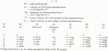
The programme for a parabolic channel of depth I and half-width W was almost identical to that used for the ellipse. Again, an 11×11 mesh was the finest that could be accommodated on the machine. Some results are in Table IIIA.

Table IIIA. Parabolic Channels

n = 3

W = half-width/depth

U ₀ = velocity at O in dimensionless form

= u ₀/{aA(ρga sin a)³

Q = discharge in dimensionless form

= q/{a ₃ A(ρga sin a)³}

U = mean velocity over the section in dimension loss form

U_s = mean velocity on the surface in dimension loss form

Table IIIB. Velocity Ratios in Parabolic Channels

u = mean velocity over the section

u_s = mean velocity on the surface

u_o = velocity at centreline or surface

D.M.O. = differential motion only

B.S.O. = bed slip only

Table IIIC. Kinematic Wave Velocities in Parabolic Channels

c = kinematic wave velocity

u = mean velocity of ice over the section

s _o = mean velocity or ice on the surface

u _o = velocity or ice at centerline or surface

D.M.O. = differential motion only

B.S.O. = bed slip only

Table IIId. Ratio of Proportional Change in Velocity to Proportional Change in Thickness for Parabolic Channels

a = ice thickness at centre or section

D.M.O. = differential motion only

B.S.O. = bed slip only

When the values of U found by horizontal and by vertical integration were compared it was found that the values on the line Y = 0 by horizontal integration were unreliable for W = 1. This is because the integration starts in the top right-hand corner where T_Z is changing rapidly. The result from vertical integration was taken as the final result for U in this case. In other cases the mean of horizontal and vertical integrations was taken. The error

shown in column 3 of Table IIIA is one-half of the maximum discrepancy between the two integrations for U (excluding the line Y = 0 when W = 1). The distributions of the velocity and shear stress are shown in Figures 8a, b, c; they are discussed in the next section.

Fig. 8a. Velocity distribution in four parabolic channels. To obtain the complete channel reflect each diagram in the left-hand boundary. n = 3

Fig. 8b. Distribution of shear-stress magnitude T (dimensionless) in parabolic channels. n = 3

Fig. 8c. Parabolic channels (n = 3). Top left: velocity on a transverse line (the Z-axis) on the surface. Top right: velocity distribution down the Y-axis. Bottom left: shear stress T_Z on the Z-axis. Bottom right: shear stress T_Y on the Y-axis. Numbers on curves are values of W

Fig. 9. Velocity U (dimensionless) on a transverse line (Z-axis) on the surface for very wide channels of rectangular, semi-elliptic and parabolic cross-section. n = 3

(Photograph by Austin S. Post, 12 August 1961)

Fig. 10. Ultramarine Glacier, Kenai Mountains, Alaska. The zone of crevasses a short distance in from the edge of the glacier indicates that the maximum shear stress does not occur at the edge itself.

Since measurements taken from the figures will be less accurate than the computed results, copies of the results for rectangles, ellipses and parabolas in numerical form have been deposited in the Library of the Glaciological Society and in the World Data Centres (Glaciology).

(iv) Discussion of results

Let us look first at the curves at the lower right in Figures 6c, 7c and 8c, which give the behaviour of T _Y on the Y axis. They are interesting because they show to what extent the linear variation for an infinitely wide channel

and for a semi-circular channel

still holds good for other channel shapes. All the curves, except that for W→∞, start out from the origin with

, a fact that experimenters using bore holes should note; Chester’s perturbation solution also gives this result, as we have already seen. The curves then bend over, but for rectangles they all meet the bed, Y = 1, with the same slope

(since the boundary condition U = 0 here implies

).

For rectangles the curves of T_Z :Z on the Z-axis (Fig. 6c, lower left) also have slope

at the origin and −1 at the edge, for the same reason. The T_Z :Z curves for ellipses and parabolas will be discussed in a moment.

For some purposes it may be useful to approximate the curve of T_Y (Y) on the Y-axis by the straight line

choosing the constant, f so as to give the true surface velocity if integration is made with this approximate shear stress up the Y-axis. The values off, which is a shape factor, are given in Table IV.

Table IV. The Shape Factor f in the Approximate Formula τ_xy = −fρg ysinα

W = half-width/depth

The velocity curves in Figures 6c, 7c, 8c at upper left show the distortion of a transverse line drawn on the glacier surface along the Z-axis. There are interesting differences between the results for rectangles, ellipses and parabolas. For rectangles (Fig. 6c) the line is always convex down glacier. For parabolas (Fig. 8c) it is convex down glacier in the centre but concave at the edges—the curvature reverses and there is a point of inflexion. This is readily explained by the behaviour of the shear-stress component T_Z (τ_zx ) on the Z-axis, which is plotted immediately below the velocity curves. T_Z is zero at the centre of the glacier, Z = 0, by symmetry. For a parabola it is also zero at the edge Z = W for the following reason. At the top right-hand corner point of the cross-section (0, W) T_Y = 0, because the upper surface is free; but the other boundary condition U = 0 on the channel wall leads to equation (15), which is.

Hence, unless , the fact that

implies T _Y = 0 at the corner (0, W). For a parabolic bed

and so T _Z − 0 at the corner. But for a rectangular or semi-elliptic bed

at the corner, and so there is no restriction of this sort on T_Z . It follows that for a parabolic channel |T_Z | must pass through a maximum at some point between the centre and the edge. This accounts for the reversal of curvature in the velocity curves for parabolas.

For the parabola with W = 1 (Fig. 8c) there is a particularly rapid change of T_Z near the edge Z = W. It is also conspicuous in the distribution of T(Y, Z) in Figure 8b. The effect is caused by the steepness of the boundary wall. As we have just remarked, if the angle ϕ of the boundary is not

, T_Z must be zero; but, if

, T_Z need not be zero. If ϕ is close to

, it is therefore quite understandable that T_Z will change rapidly from a comparatively high value a short distance from the edge to zero on the edge itself.

If one were tempted to guess from the above arguments that there would he no maximum in |T_Z | on the surface for semi-elliptic channels, one would be wrong. Figure 7c shows that |T_Z | does go through a maximum for elliptic channels when W = 3 and also when W = 4. For W = 2 it probably does not. For W = 1 it certainly does not, and Chester’s solution shows that it does not for small departures from W = 1. Why should |T_Z | behave like this for elliptic channels? The reason is seen by letting W become very large. Then on any line, Z = constant in the YZ plane, not too close to the edge, the velocity distribution will be that of an infinitely wide channel of appropriate depth. The surface velocity U is therefore proportional to H ⁴, where H is the depth below the point in question. If we plot the curve of U against. Z/W on this basis for a semi-ellipse (Fig. 9) it is found to have an inflexion at Z/W = 1/√3 = 0.577 (shown by an arrow). The corresponding curve for a parabola has an inflexion at, Z/W = 1/√7 = 0.378. The curve for a rectangle is simply the straight line

and has no inflexion. An inflexion in the U curve means a maximum of |T_Z |. The fact that |T_Z | shows a maximum for elliptic channels at the higher values of W is thus understandable.Footnote *

The channels of real glaciers are nearly always sloping, not vertical, at the edges. To the extent that there is no slip on the bed the arguments for τ_zx = T_Z = 0 at the edge will therefore apply. So we must expect that the maximum shear stress in the surface of a glacier will not occur precisely at the edge but at a certain distance in. If there is a gap between the glacier and the rock wall T_Z will certainly be zero at the extreme edge. Thus, curiously enough, no slip and free slip give the same result.

Observation confirms that the maximum shear stress is not always at the edge. To give one example: at a transverse line of stakes on Austerdalsbreen, Norway, over three different periods of observation, 1957–58, 1958–59 and 1958–63 a reversal of curvature (point of inflexion) occurred consistently at Z = −0.7W. The slope of the side wall on that side was ϕ = 33°. At the other end of the same line ϕ was much greater, 62°; for 1957–58 no inflexion was detected, but there was an observable inflexion for both 1958–59 and 1958–63 between Z = 0.9 and Z = W. In other words, the steeper the side wall the closer is the inflexion, as the theoretical discussion leads us to expect. Since it occurs rather close to the glacier edge, perhaps in a lateral moraine, the inflexion phenomenon may often pass undetected. Figure ro shows evidence of the same effect on Ultramarine Glacier, Kenai Mountains, Alaska, in the form of a zone of marginal crevasses which occur a short distance in from the ice edge (the photograph is by Austin S. Post, who has kindly given permission to reproduce it). This phenomenon explains why one can sometimes find a way down a glacier by going to the extreme margin when progress a short distance in from the edge is blocked by crevasses.

Let us now look at the distributions of T(Y, Z) in Figures 6b, 7b, 8b. The fact that, for W > 1, |T_Z | may have a maximum on the Z-axis, but that |T_Y | has no maximum on the Y-axis, accounts for the general nature of the distributions. For the rectangles with W = 2 and 3 the pattern of T(Y, Z) near the side wall is very similar; it suggests that there is a rather constant “edge effect” for wide channels. An invariable rule for all the channels is that the highest shear stress occurs at the point of the bed closest to the origin. For W > 1 this point is always the centre of the bed, except in the one case of parabolas with W near to 1; Figure 8b (W = 1) illustrates this.

Figure 11 shows the centre-line velocity U ₀ plotted against W for all three channel shapes. The curves for rectangles and ellipses, but not parabolas, should obey the similarity principles of §4. The tangents at the points W = 1 on the curves are drawn through the point

on the W axis, and it is interesting to see how closely the curves follow the tangents even up to W = 2. In closing this discussion let us emphasize the great effect that the drag of the valley sides has on the centre-line velocity. In a parabolic valley with a ratio of width to depth of 8(W = 4) the centre-line velocity is approximately half what it would be in an infinitely wide valley of the same depth (Fig. 11); Table IIIA gives the factor as 0.131/0.250 = 0.524.

Fig. 11. Velocity U₀ (dimensionless) at the origin as a function of W, the ratio of half-width to depth, for rectangular, semi-elliptic and parabolic channels. n = 3

7. Discharge and Mean Velocities

By integrating the velocity over the cross-section we may find the discharge q. This is given in the dimensionless form

(18)

in Tables II and IIIA. Since the parabolic bed is closest to the real situation in glaciers our further discussions are concerned with this case.

Q is plotted against Win Figure 12 for n = 3. The two extreme cases W→0 and W→∞ may be treated analytically. As W→0 the velocity distribution on any horizontal line becomes the same as that in an infinitely deep channel of appropriate width. By this principle we find, for a parabolic bed, as W→0,

Fig. 12. Discharge Q (dimensionless) for parabolic channels as a function of W. n = 3

or, for n = 3, Q→(4/35)W ⁵. On the other hand, as W→0 the velocity distribution on any vertical line where the depth is H, say, is the same as that in an infinitely wide channel of uniform depth H. By this principle we obtain for a parabolic bed,

where

(19)

with

Putting n = 3 we find

Hence the Q:W curve has an asymptotic slope of

(The Q value for W = 4 is thereby improved from 0.41 to 0.404.)

The mean velocity over the section, u , is given in dimensionless form

by

As W→0,

The mean velocity along a transverse line drawn on the glacier surface is also of interest because it is relati.re. Call it u _s , or in dimensionless form

It is given, for n = 3, in column 7 of Table IIIA. The principles used above lead to the result that as W→0, U _s →(n+2)⁻¹ W ⁿ⁺¹, and, as W→∞, U _s →(n+1)⁻¹ I(2n+3).

Table IIIA shows that, for W > 2 and n = 3, U _s is quite close to U . The ratio

What effect will slip on the bed have on this last result? Apparently, very little. For suppose that the entire motion consisted of bed slip, so that the glacier moved forward as a rigid body. Then certainly the ratio

It may be asked how sensitive this result for n = 3 is to the value of n. Velocity distributions for n≠3 have not been computed, but nevertheless some information on the n dependence may be obtained by the following argument. In the extreme case W→0 we find from previous results

and for W→0

by the recurrence relation (19). Thus, for these two extreme cases we know precisely how the ratio u /u_s depends on n. In Table IIIB, columns 2 and 6 show the values calculated for the two extreme cases with n = 2 and 4. The variation of

The values of u /u_s , that would occur if motion consisted entirely of bed slip are all equal to t and are shown in Table IIIB under the heading B.S.O. (bed slip only). We conclude from the table that u equals u _s to within a few per cent for 2 > W > 4 regardless of the amount of bed slip, and even when n differs a little from 3.

The ratios u /u_s , and u _s /u ₀ are also shown in Table IIIB for n = 3 for differential motion only and for bed slip only. The values for W→0 and W→∞W are respectively

and

Estimates for n = 2 and n = 4 at intermediate values of W have been made accordingly. It will be seen that the ratios are quite insensitive to the value of n, but, unlike u /u_s , they may be expected to vary significantly with the amount of bed slip.

8. Kinematic Wave Velocity

It is shown in Lighthill and Whitham (1955) or Nye (1960) that for unsteady slow flow in a channel the velocity of kinematic waves of constant q is given by

where S is the area of cross-section. This means that if the level of the ice in a fixed parabolic channel changes so as to increase the cross-sectional area of the ice by dS, the discharge will increase by dq, and the ratio gives the kinematic wave velocity. Clearly, our computations on parabolic sections contain the necessary information to find c for n = 3, but a little further thought is needed because the calculations have explicitly referred to a channel of fixed depth and variable width, rather than a variable height of ice surface in a fixed channel. We proceed as follows, for general n, remembering that differentiations with respect to S are for a fixed parabola.

By the definition of Q = Q(W) in (18) we have q = Q(W) γ(a), where γ(a) ∝ a ⁿ⁺³. Therefore

But, for a fixed parabola,

For n = 3 we take the values of dQ/dW from the graph of Q:W (Fig. 12) and so calculate c/ u (Table IIIC, under the heading n = 3, D.M.O., c/ u ). As W→0 we have seen that Q→{4/(n+2) (n+4)}W ⁿ⁺², which leads to

Let us now consider the effect on the ratio c/ u of bed slip and of changing n. To estimate the effect of bed slip it is instructive to think once again about the case where motion is entirely due to slip on the bed, there being no differential motion within the ice at all. We assume that slip occurs according to the law

where τ _b , is the shear stress on the bed, and

c/u calculated with this formula and n = 2, 3 and 4 is given in Table IIIC under the heading c/ u , B.S.O. It seems plausible to expect that when motion is partly due to bed slip and partly to differential motion within the ice the ratio c/ u will lie between the extremes calculated for D.M.O. and B.S.O.

The effect on the ratio c/ u of changing n is estimated by the method used before: we know precisely how the ratio depends on n for W→0 and W→∞, so we use this information to make a rough estimate of the effect at intermediate W. The values of c/ u in Table IIIC show how this ratio is affected both by bed slip and by a change of n.

The values of c/u ₀ and c/u _s in Table IIIc now follow in a straightforward way. The forms for W→0 and W→∞ respectively are

and

Of the three ratios, c/ u , c/u ₀ and c/u _s, the one shown by Table IIIC to be least affected by the amount of bed slip is c/u ₀. It happens that this is also the ratio that is least dependent on W over the practically important range 1 < W < 4. Indeed for this range of W and for n = 3 c/u ₀ lies between 2.0 and 2.3 regardless of the amount of bed slip. The ratio goes up or down by about 0.3 as n increases or decreases by 1. In practical cases where the amount of bed slip is unknown this ratio c/u ₀, seems to be the most useful.

Effect of changes in thickness on the velocity. One further type of ratio may be considered. Since

Since c/ u is already known, this formula enables us to find

The fractional change in the centre-line velocity is also of interest. Remembering that the changes are those for a fixed channel, some differentiation similar to that used above in finding c/ u shows that

For n = 3, dU ₀/dW is taken from the graph of U ₀: W in Figure 11, and the resulting values of (a/u ₀)(du ₀/da) are shown in Table IIID under the heading n = 3, D.M.O. The values when there is bed slip only (B.S.O.) are of course the same as those of

The ratio (a/u _s )(du _s /da) is formed in a similar way. For the case of differential motion only it is notable that the formulae for W→0 and W→∞ are exactly the same for u , u ₀ and u _s , namely

By way of summary we may pick out the following leading results from Tables IIIB, C and D. (1) The average surface velocity u _s is equal to the average velocity over the section u to within a few per cent for 2<W<4 regardless of the relative contribution of bed slip. This result is most exact for n = 3 but is not sensitive to the precise value of n. (2) For 1  < W < 4 and n = 3, the kinematic wave velocity c is between 2.0 and 2.3 times the centre-line velocity of the ice u ₀ regardless of the amount of bed slip. This ratio goes up or down by about 0.3 as n increases or decreases by 1. (3) For 1 < W < 4 and n = 3, c is between 2.0 and 3.5 times the mean surface velocity of the ice u _s . The exact value depends on W and on the amount of bed slip, and changes by up to 0.8 as n changes by 1. (4) The ratio of the fractional change in velocity to a given fractional change in ice thickness is only slightly dependent on which velocity is specified; but it can take values ranging from 1.1 [to 4.7 depending on the amount of bed slip, the width-depth ratio (1 < W < 4), and the value of n (2 < n< 4).

9. Acknowledgements

The computations were done on the I.B.M. 1620 machine of the Computer Unit, Bristol University. I should like to thank Dr. M. H. Rogers, in charge of the Computer Unit, for his very helpful guidance on computational methods.