


1 Introduction
The surface-piercing flap-type oscillating wave surge converters (OWSCs) are among the most efficient devices to extract energy from water waves (Babarit et al. Reference Babarit, Hals, Muliawan, Kurniawan, Moan and Krokstad2012). These devices consist of buoyant flaps hinged on a bottom foundation and move back and forth as an inverted pendulum under the action of the waves. A power take-off (PTO) mechanism converts the gate motion into electricity. Because of their ability to capture energy with large efficiency, these converters have received significant attention in recent years, leading to analytical theories (Linton & McIver Reference Linton and McIver2001; Mei, Stiassnie & Yue Reference Mei, Stiassnie and Yue2005) and experimental campaigns (Folley, Whittaker & van’t Hoff Reference Folley, Whittaker and van’t Hoff2007; Henry et al. Reference Henry, Doherty, Cameron, Whittaker and Doherty2010). Renzi & Dias (Reference Renzi and Dias2012, Reference Renzi and Dias2013, Reference Renzi and Dias2014) have developed a semi-analytical theory based on a hypersingular integral equation approach to investigate the hydrodynamic behaviour of a ‘thin gate’ in a channel and in open sea. Michele et al. (Reference Michele, Sammarco, d’Errico, Renzi, Abdolali, Bellotti and Dias2015) and Michele, Sammarco & d’Errico (Reference Michele, Sammarco and d’Errico2016a ) have extended the theory of Renzi & Dias (Reference Renzi and Dias2013) to the case of a single and multiple arrays of neighbouring OWSCs with finite thickness in open sea and in front of a vertical breakwater. Recently, Michele, Sammarco & d’Errico (Reference Michele, Sammarco and d’Errico2016b ) devised an analytical theory which describes the wave field and gate motion in terms of elliptic coordinates and Mathieu functions, while Sarkar, Doherty & Dias (Reference Sarkar, Doherty and Dias2016) solved the case of a finite array of cylindrical OWSCs.
The vast majority of existing analytical theories have been developed within the framework of linear theories for small amplitude oscillations. However, neglecting nonlinear effects is unjustified in some practical cases and might cause us to overlook constructive resonance phenomena. In this paper we describe a nonlinear theory for the hydrodynamic behaviour of a single array of several floating flap-gate OWSCs hinged on a fixed, rigid and fully reflecting wall. The gates oscillate under the action of the incident waves and an appropriate PTO located at the hinge converts the mechanical energy into electricity and returns a resistant torque. We consider the gates spanning the full width of an infinitely long channel. Due to the mirroring effect of the channel walls we thus model the behaviour of an infinite array of converters. In this case, the natural modes can be completely trapped with no radiation damping. Trapped modes are of considerable interest in several contexts such as acoustic waves (Hein & Koch Reference Hein and Koch2008), quantum waveguides (Linton & Ratcliffe Reference Linton and Ratcliffe2004), elastic waves (Porter Reference Porter2007) and electromagnetic waves (Porter & Evans Reference Porter and Evans1999). For water waves, Evans & Linton (Reference Evans and Linton1991) derived the wave field of trapped modes around a fixed vertical cylinder, while in coastal oceanography the wave trapping of edge waves on a sloping beach is well known (Blondeaux & Vittori Reference Blondeaux and Vittori1995; Mei et al. Reference Mei, Stiassnie and Yue2005; Li Reference Li2007). In the case of neighbouring articulated gates Li & Mei (Reference Li and Mei2003) developed a mathematical theory to determine all the out-of-phase trapped modes of an array of gates in an infinitely long channel; Sammarco, Michele & d’Errico (Reference Sammarco, Michele and d’Errico2013) solved the case of multiple arrays of gates hydrodynamically coupled.
Trapped modes cannot be synchronously resonated in a linearized framework. This is because the modal matrix and the forcing terms are orthogonal (Adamo & Mei Reference Adamo and Mei2005). For this reason, resonance of trapped modes is possible only through a nonlinear mechanism. Guza & Bowen (Reference Guza and Bowen1976) and Rockliff (Reference Rockliff1978) have shown that trapped edge waves can be resonated subharmonically by incident waves with frequency twice the natural frequency of the edge wave. Li & Mei (Reference Li and Mei2006) have developed a nonlinear theory to analyse the subharmonic resonance of trapped surface waves around a fixed cylinder while Lichter & Chen (Reference Lichter and Chen1987) analysed the resonance of nonlinear cross-waves in a long channel. A similar subharmonic mechanism has been analysed for the so-called ‘Faraday resonance’: for the main contributions we refer to Miles (Reference Miles1984a ), Holmes (Reference Holmes1986), Gu & Sethna (Reference Gu and Sethna1987) and Miles & Henderson (Reference Miles and Henderson1990). Of considerable engineering interest is the case of mobile neighbouring gates to protect Venice from flooding. Laboratory experiments have revealed that, for certain frequencies, the incident waves resonate subharmonically the trapped modes of the barrier (Mei et al. Reference Mei, Sammarco, Chan and Procaccini1994). The weakly nonlinear theory which explains this resonance mechanism has been developed by Sammarco, Tran & Mei (Reference Sammarco, Tran and Mei1997a ), Sammarco et al. (Reference Sammarco, Tran, Gottlieb and Mei1997b ) for uniform and modulated waves. A simplified model for the subharmonic resonance of sliding gates in shallow waters has been developed by Vittori, Blondeaux & Seminara (Reference Vittori, Blondeaux and Seminara1996).
In the present paper we extend the theory of Sammarco et al. (Reference Sammarco, Tran and Mei1997a ,Reference Sammarco, Tran, Gottlieb and Mei b ) to investigate the hydrodynamics of the array of OWSCs. By considering small height of the gates with respect to the water depth, a simplified version of the governing equations and then for the coefficient of the evolution equation is found, with a new term that accounts for energy extraction. First, we consider subharmonic excitation of a single mode. We derive the complex nonlinear evolution equation of the Stuart–Landau form (Aranson & Kramer Reference Aranson and Kramer2002) which describes the dynamical growth of the resonated trapped mode. A parametric analysis of the coupling coefficients in terms of the array characteristics is carried out. The case of uniform incident waves points out the dependence of the bandwidth of instability, the resonated amplitude and the thresholds of resonance on the PTO coefficient. The generated power due to the subharmonic resonance of the natural modes is then evaluated. We find the optimal value of the PTO coefficient which maximizes power extraction and show that subharmonic excitation yields constructive interactions in terms of power extraction. We obtain that the capture factor is larger than the theoretical maximum of a two-dimensional absorber in a infinite long channel within the linear theory (Mei et al. Reference Mei, Stiassnie and Yue2005).
For modulated waves, we find period doubling sequences, chaotic states and frequency downshift (Trulsen & Mei Reference Trulsen and Mei1995; Trulsen & Dysthe Reference Trulsen and Dysthe1997; Sammarco et al. Reference Sammarco, Tran, Gottlieb and Mei1997b ) by increasing the modulated wave amplitude. We detect the occurrence of homoclinic tangles and global chaos through usage of the Melnikov function (Guckenheimer & Holmes Reference Guckenheimer and Holmes1983; Jordan & Smith Reference Jordan and Smith2011). Extensive parametric analysis is then performed to study the effects of the chaotic behaviour on the generated power and efficiency. We show that chaotic motion of the gates decreases the efficiency in terms of energy production; a deterministic confirmation of the previous findings of Michele et al. (Reference Michele, Sammarco and d’Errico2016a ,Reference Michele, Sammarco and d’Errico b ) for gate energy production under stochastic incident wave spectra.
Next, we examine the competition of two modes assuming the incident wave frequency equal to the summation of the respective eigenfrequencies (Nayfeh & Mook Reference Nayfeh and Mook1995). Quadratic interactions at higher orders generate several harmonics. This nonlinear coupling leads to triad interactions and energy transfer between trapped modes. Interesting phenomena involving triad interactions have been studied in the context of acoustic–gravity waves (Kadri & Stiassnie Reference Kadri and Stiassnie2013; Kadri & Akylas Reference Kadri and Akylas2016), edge waves (Li Reference Li2007), Bragg scattering by bottom ripples (Mei et al. Reference Mei, Stiassnie and Yue2005) and interfacial waves (Alam Reference Alam2012), while contributions to the analysis of mode–mode interactions can be found in Mei & Zhou (Reference Mei and Zhou1991) and Zardi & Seminara (Reference Zardi and Seminara1995) for pulsating bubbles and Ciliberto & Gollub (Reference Ciliberto and Gollub1985), Simonelli & Gollub (Reference Simonelli and Gollub1989), Kambe & Umeki (Reference Kambe and Umeki1990), Umeki (Reference Umeki1991) for Faraday waves. The coupled evolution equations of both modal amplitudes are obtained and now involve coupling terms. Similarly to the case of single subharmonic resonance we derive the bifurcation diagrams to analyse the effects of the incident wave phase shift on the equilibrium and unstable states. The contribution due to mode–mode coupling on the OWSCs efficiency is finally given. We show that mode–mode coupling yields constructive interactions in terms of generated power but less pronounced than the pure subharmonic resonance of a single mode.
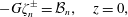
Figure 1. Plan geometry of the array and side view of the gate in physical variables. The OWSCs do not span the entire water depth but are placed upon a vertical fixed wall on a rigid bottom.
2 Governing equations
A sketch representing the array of floating OWSCs hinged upon a fixed, rigid and fully reflecting wall is depicted in figure 1. We indicate the physical variables by primes. The figure shows identical gates of width
 $a^{\prime }$
and thickness
$a^{\prime }$
and thickness
 $2d^{\prime }$
in an infinite straight long channel of width
$2d^{\prime }$
in an infinite straight long channel of width
 $b^{\prime }$
. Let
$b^{\prime }$
. Let
 $h^{\prime }$
and
$h^{\prime }$
and
 $c^{\prime }$
denote respectively the channel depth and the wall height; also
$c^{\prime }$
denote respectively the channel depth and the wall height; also
 $h_{p}^{\prime }=h^{\prime }-c^{\prime }$
is the distance from the free surface to the hinge with
$h_{p}^{\prime }=h^{\prime }-c^{\prime }$
is the distance from the free surface to the hinge with
 $h_{p}^{\prime }\ll h^{\prime }$
(or
$h_{p}^{\prime }\ll h^{\prime }$
(or
 $c^{\prime }\sim h^{\prime }$
). Define a Cartesian reference system with the
$c^{\prime }\sim h^{\prime }$
). Define a Cartesian reference system with the
 $x^{\prime }$
and
$x^{\prime }$
and
 $y^{\prime }$
-axes lying on the mean free surface and the
$y^{\prime }$
-axes lying on the mean free surface and the
 $z^{\prime }$
-axis pointing vertically upward. The
$z^{\prime }$
-axis pointing vertically upward. The
 $y^{\prime }$
-axis bisects the array, while the
$y^{\prime }$
-axis bisects the array, while the
 $x^{\prime }$
-axis coincides with the left bank of the channel. The gates oscillate about a common axis located at
$x^{\prime }$
-axis coincides with the left bank of the channel. The gates oscillate about a common axis located at
 $z^{\prime }=-h^{\prime }+c^{\prime }=-h_{p}^{\prime }$
,
$z^{\prime }=-h^{\prime }+c^{\prime }=-h_{p}^{\prime }$
,
 $x^{\prime }=0$
. Assume that the incoming waves come from
$x^{\prime }=0$
. Assume that the incoming waves come from
 $x\rightarrow +\infty$
and are normally incident to the gates. Let
$x\rightarrow +\infty$
and are normally incident to the gates. Let
 $G_{q}$
,
$G_{q}$
,
 $q=1,\ldots ,Q$
, denote the
$q=1,\ldots ,Q$
, denote the
 $q$
th gate and
$q$
th gate and
 $\unicode[STIX]{x1D6E9}_{q}^{\prime }$
be the angular displacement of
$\unicode[STIX]{x1D6E9}_{q}^{\prime }$
be the angular displacement of
 $G_{q}$
, then we can define
$G_{q}$
, then we can define
 $\unicode[STIX]{x1D6E9}^{\prime }(y,t)=\{\unicode[STIX]{x1D6E9}_{1}^{\prime }(t),\ldots ,\unicode[STIX]{x1D6E9}_{q}^{\prime }(t),\ldots ,\unicode[STIX]{x1D6E9}_{Q}^{\prime }(t)\}$
as the angular displacement function of the array. The fluid is assumed to be inviscid and incompressible and the flow irrotational, hence the velocity field satisfies the Laplace equation in the fluid domain
$\unicode[STIX]{x1D6E9}^{\prime }(y,t)=\{\unicode[STIX]{x1D6E9}_{1}^{\prime }(t),\ldots ,\unicode[STIX]{x1D6E9}_{q}^{\prime }(t),\ldots ,\unicode[STIX]{x1D6E9}_{Q}^{\prime }(t)\}$
as the angular displacement function of the array. The fluid is assumed to be inviscid and incompressible and the flow irrotational, hence the velocity field satisfies the Laplace equation in the fluid domain
 $\unicode[STIX]{x1D6FA}$
:
$\unicode[STIX]{x1D6FA}$
:
 $$\begin{eqnarray}\unicode[STIX]{x1D6FB}^{\prime 2}\unicode[STIX]{x1D6F7}^{\prime }(x^{\prime },y^{\prime },z^{\prime })=0\quad (x^{\prime },y^{\prime },z^{\prime })\in \unicode[STIX]{x1D6FA}.\end{eqnarray}$$
Let
 $A_{T}^{\prime }$
be the amplitude of the free-surface oscillations,
$A_{T}^{\prime }$
be the amplitude of the free-surface oscillations,
 $\unicode[STIX]{x1D706}^{\prime }$
the wavelength,
$\unicode[STIX]{x1D706}^{\prime }$
the wavelength,
 $\unicode[STIX]{x1D714}^{\prime }$
the eigenfrequency of the natural mode and
$\unicode[STIX]{x1D714}^{\prime }$
the eigenfrequency of the natural mode and
 $g^{\prime }$
the acceleration due to gravity. Then introduce the following non-dimensional quantities:
$g^{\prime }$
the acceleration due to gravity. Then introduce the following non-dimensional quantities:
 $$\begin{eqnarray}\left.\begin{array}{@{}c@{}}(x,y,z)=(x^{\prime },y^{\prime },z^{\prime })/\unicode[STIX]{x1D706}^{\prime },\quad \unicode[STIX]{x1D6F7}=\unicode[STIX]{x1D6F7}^{\prime }/A_{T}^{\prime }\unicode[STIX]{x1D714}^{\prime }\unicode[STIX]{x1D706}^{\prime },\quad \unicode[STIX]{x1D701}=\unicode[STIX]{x1D701}^{\prime }/A_{T}^{\prime },\quad t=t^{\prime }\unicode[STIX]{x1D714}^{\prime },\\ (b,c)=(b^{\prime },c^{\prime })/\unicode[STIX]{x1D706}^{\prime },\quad d=d^{\prime }/h_{p}^{\prime },\quad h=h^{\prime }/\unicode[STIX]{x1D706}^{\prime },\quad \unicode[STIX]{x1D6E9}^{\prime }=\unicode[STIX]{x1D6E9}A_{T}^{\prime }/h_{p}^{\prime },\quad G=g^{\prime }/\unicode[STIX]{x1D714}^{\prime 2}\unicode[STIX]{x1D706}^{\prime },\end{array}\right\}\quad\end{eqnarray}$$
where
 $\unicode[STIX]{x1D701}^{\prime }$
is the free-surface elevation and
$\unicode[STIX]{x1D701}^{\prime }$
is the free-surface elevation and
 $G$
the non-dimensional eigenfrequency. We introduce the following two length ratios to be smaller than unity:
$G$
the non-dimensional eigenfrequency. We introduce the following two length ratios to be smaller than unity:
 $$\begin{eqnarray}\unicode[STIX]{x1D716}=A_{T}^{\prime }/h_{p}^{\prime }\ll 1,\quad \unicode[STIX]{x1D707}=h_{p}^{\prime }/\unicode[STIX]{x1D706}^{\prime }\ll 1.\end{eqnarray}$$
With the introduction of these two small parameters the formulation of the problem becomes algebraically simpler to Sammarco et al. (Reference Sammarco, Tran and Mei1997a
). Indeed, let
 $\unicode[STIX]{x1D6FA}^{+}\,(\unicode[STIX]{x1D6FA}^{-})$
denote the fluid regions to the right (left) of the gates and distinguish physical quantities in
$\unicode[STIX]{x1D6FA}^{+}\,(\unicode[STIX]{x1D6FA}^{-})$
denote the fluid regions to the right (left) of the gates and distinguish physical quantities in
 $\unicode[STIX]{x1D6FA}^{\pm }$
through
$\unicode[STIX]{x1D6FA}^{\pm }$
through
 $\pm$
. Laplace and Bernoulli equations read
$\pm$
. Laplace and Bernoulli equations read
 $$\begin{eqnarray}\displaystyle & \displaystyle \unicode[STIX]{x1D6FB}^{2}\unicode[STIX]{x1D6F7}^{\pm }=0, & \displaystyle\end{eqnarray}$$
 $$\begin{eqnarray}\displaystyle & \displaystyle -\frac{p^{\prime \pm }}{\unicode[STIX]{x1D70C}\unicode[STIX]{x1D714}^{\prime ^{2}}\unicode[STIX]{x1D706}^{\prime 2}}=Gz+\unicode[STIX]{x1D716}\unicode[STIX]{x1D707}\unicode[STIX]{x1D6F7}_{t}^{\pm }+\unicode[STIX]{x1D716}^{2}\unicode[STIX]{x1D707}^{2}\frac{1}{2}|\unicode[STIX]{x1D735}\unicode[STIX]{x1D6F7}^{\pm }|^{2}, & \displaystyle\end{eqnarray}$$
the dynamic and mixed boundary condition on the free surface are respectively
 $$\begin{eqnarray}-G\unicode[STIX]{x1D701}=\unicode[STIX]{x1D6F7}_{t}^{\pm }+\unicode[STIX]{x1D716}\unicode[STIX]{x1D707}{\textstyle \frac{1}{2}}|\unicode[STIX]{x1D735}\unicode[STIX]{x1D6F7}^{\pm }|^{2},\quad z=\unicode[STIX]{x1D716}\unicode[STIX]{x1D707}\unicode[STIX]{x1D701},\end{eqnarray}$$
 $$\begin{eqnarray}\unicode[STIX]{x1D6F7}_{tt}^{\pm }+G\unicode[STIX]{x1D6F7}_{z}^{\pm }+\unicode[STIX]{x1D716}\unicode[STIX]{x1D707}|\unicode[STIX]{x1D735}\unicode[STIX]{x1D6F7}^{\pm }|_{t}^{2}+\unicode[STIX]{x1D716}^{2}\unicode[STIX]{x1D707}^{2}{\textstyle \frac{1}{2}}\unicode[STIX]{x1D735}\boldsymbol{\cdot }\unicode[STIX]{x1D735}|\unicode[STIX]{x1D735}\unicode[STIX]{x1D6F7}^{\pm }|^{2}=0,\quad z=\unicode[STIX]{x1D716}\unicode[STIX]{x1D707}\unicode[STIX]{x1D701},\end{eqnarray}$$
while the no-flux conditions at the bottom and channel walls require
 $$\begin{eqnarray}\unicode[STIX]{x1D6F7}_{z}^{\pm }=0,\quad z=-h,\end{eqnarray}$$
 $$\begin{eqnarray}\unicode[STIX]{x1D6F7}_{y}^{\pm }=0,\quad y=0\quad \text{and}\quad y=b.\end{eqnarray}$$
The kinematic condition on the surface of the array
 $$\begin{eqnarray}x=\unicode[STIX]{x1D709}^{\pm }=\left[-(z+\unicode[STIX]{x1D707})\tan \unicode[STIX]{x1D716}\unicode[STIX]{x1D6E9}\pm \unicode[STIX]{x1D707}\frac{d}{\cos ^{2}\unicode[STIX]{x1D6E9}}\right]H(z+h-c)\pm \unicode[STIX]{x1D707}\,dH(-z-h+c),\end{eqnarray}$$
can be written as
 $$\begin{eqnarray}\unicode[STIX]{x1D6F7}_{x}^{\pm }=\left\{\unicode[STIX]{x1D6E9}_{t}\left[-\frac{(z+\unicode[STIX]{x1D707})}{\unicode[STIX]{x1D707}\cos ^{2}\unicode[STIX]{x1D716}\unicode[STIX]{x1D6E9}}\pm \frac{d\sin \unicode[STIX]{x1D716}\unicode[STIX]{x1D6E9}}{\cos ^{2}\unicode[STIX]{x1D716}\unicode[STIX]{x1D6E9}}\right]-\unicode[STIX]{x1D6F7}_{z}^{\pm }\tan \unicode[STIX]{x1D716}\unicode[STIX]{x1D6E9}\right\}H(z+h-c),\end{eqnarray}$$
where
 $H$
denotes the Heaviside step function.
$H$
denotes the Heaviside step function.
Let us introduce a new pair of coordinates
 $(y_{1},z_{1})=(y^{\prime },z^{\prime })/h_{p}^{\prime }=(y,z)/\unicode[STIX]{x1D707}$
. The equation of motion of the
$(y_{1},z_{1})=(y^{\prime },z^{\prime })/h_{p}^{\prime }=(y,z)/\unicode[STIX]{x1D707}$
. The equation of motion of the
 $q$
th gate coupled with an energy generator at the hinge is given by
$q$
th gate coupled with an energy generator at the hinge is given by
 $$\begin{eqnarray}\displaystyle & & \displaystyle I\unicode[STIX]{x1D716}\unicode[STIX]{x1D6E9}_{q,tt}-GS\sin \unicode[STIX]{x1D716}\unicode[STIX]{x1D6E9}_{q}+\overline{\unicode[STIX]{x1D708}}_{pto}\unicode[STIX]{x1D716}\unicode[STIX]{x1D6E9}_{q,t}\nonumber\\ \displaystyle & & \displaystyle \quad =-\,\int _{((q-1)a)/\unicode[STIX]{x1D707}}^{(qa)/\unicode[STIX]{x1D707}}\,\text{d}y_{1}\left\{\int _{-1}^{\unicode[STIX]{x1D716}\unicode[STIX]{x1D701}^{+}}\,\text{d}z_{1}\left(Gz_{1}+\unicode[STIX]{x1D716}\unicode[STIX]{x1D6F7}_{t}^{+}+\unicode[STIX]{x1D716}^{2}\unicode[STIX]{x1D707}\frac{1}{2}|\unicode[STIX]{x1D735}\unicode[STIX]{x1D6F7}^{+}|^{2}\right)\frac{z_{1}+1-d\sin \unicode[STIX]{x1D716}\unicode[STIX]{x1D6E9}_{q}}{\cos ^{2}\unicode[STIX]{x1D716}\unicode[STIX]{x1D6E9}_{q}}\right.\nonumber\\ \displaystyle & & \displaystyle \left.\qquad -\,\int _{-1}^{\unicode[STIX]{x1D716}\unicode[STIX]{x1D701}^{-}}\,\text{d}z_{1}\left(Gz_{1}+\unicode[STIX]{x1D716}\unicode[STIX]{x1D6F7}_{t}^{-}+\unicode[STIX]{x1D716}^{2}\unicode[STIX]{x1D707}\frac{1}{2}|\unicode[STIX]{x1D735}\unicode[STIX]{x1D6F7}^{-}|^{2}\right)\frac{z_{1}+1+d\sin \unicode[STIX]{x1D716}\unicode[STIX]{x1D6E9}_{q}}{\cos ^{2}\unicode[STIX]{x1D716}\unicode[STIX]{x1D6E9}_{q}}\right\}+O(\unicode[STIX]{x1D716}^{4}),\nonumber\\ \displaystyle & & \displaystyle\end{eqnarray}$$
where
 $I=I^{\prime }/\unicode[STIX]{x1D70C}h_{p}^{\prime 4}\unicode[STIX]{x1D706}^{\prime }$
is the non-dimensional inertia of the gate about the hinge,
$I=I^{\prime }/\unicode[STIX]{x1D70C}h_{p}^{\prime 4}\unicode[STIX]{x1D706}^{\prime }$
is the non-dimensional inertia of the gate about the hinge,
 $S=S^{\prime }/\unicode[STIX]{x1D70C}h_{p}^{\prime 4}$
the non-dimensional first moment of the gate,
$S=S^{\prime }/\unicode[STIX]{x1D70C}h_{p}^{\prime 4}$
the non-dimensional first moment of the gate,
 $\overline{\unicode[STIX]{x1D708}}_{pto}=\unicode[STIX]{x1D708}_{pto}^{\prime }/A_{T}^{2}\unicode[STIX]{x1D714}\unicode[STIX]{x1D70C}h_{p}^{2}\unicode[STIX]{x1D706}$
the non-dimensional power take-off coefficient. Typical values of
$\overline{\unicode[STIX]{x1D708}}_{pto}=\unicode[STIX]{x1D708}_{pto}^{\prime }/A_{T}^{2}\unicode[STIX]{x1D714}\unicode[STIX]{x1D70C}h_{p}^{2}\unicode[STIX]{x1D706}$
the non-dimensional power take-off coefficient. Typical values of
 $\unicode[STIX]{x1D708}_{pto}^{\prime }$
are
$\unicode[STIX]{x1D708}_{pto}^{\prime }$
are
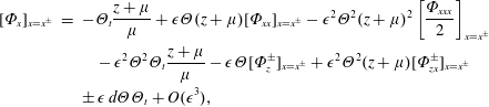
 $10^{2}{-}10^{3}~\text{kg}~\text{m}^{2}~\text{s}^{-1}$
, so that for typical conditions
$10^{2}{-}10^{3}~\text{kg}~\text{m}^{2}~\text{s}^{-1}$
, so that for typical conditions
 $A_{T}^{2}=O(0.1)~\text{m}$
,
$A_{T}^{2}=O(0.1)~\text{m}$
,
 $\unicode[STIX]{x1D714}=O(1)~\text{rad}~\text{s}^{-1}$
,
$\unicode[STIX]{x1D714}=O(1)~\text{rad}~\text{s}^{-1}$
,
 $h_{p}^{2}=O(10)~\text{m}$
,
$h_{p}^{2}=O(10)~\text{m}$
,
 $\unicode[STIX]{x1D706}=O(10){-}O(10^{2})~\text{m}$
, we obtain
$\unicode[STIX]{x1D706}=O(10){-}O(10^{2})~\text{m}$
, we obtain
 $\overline{\unicode[STIX]{x1D708}}_{pto}=O(10^{-2})$
. Hence we assume
$\overline{\unicode[STIX]{x1D708}}_{pto}=O(10^{-2})$
. Hence we assume
 $\overline{\unicode[STIX]{x1D708}}_{pto}=\unicode[STIX]{x1D716}^{2}\unicode[STIX]{x1D708}_{pto}$
. Note that usage of the coordinates
$\overline{\unicode[STIX]{x1D708}}_{pto}=\unicode[STIX]{x1D716}^{2}\unicode[STIX]{x1D708}_{pto}$
. Note that usage of the coordinates
 $(y_{1},z_{1})$
renders
$(y_{1},z_{1})$
renders
 $O(1)$
the interval of the integrals in (2.12) and allows us to evaluate appropriately the order of magnitude of each term inside the integrand. Therefore, in the above expression (2.12) the contribution due to the PTO torque on the gate motion results small; indeed the term is
$O(1)$
the interval of the integrals in (2.12) and allows us to evaluate appropriately the order of magnitude of each term inside the integrand. Therefore, in the above expression (2.12) the contribution due to the PTO torque on the gate motion results small; indeed the term is
 $O(\unicode[STIX]{x1D716}^{3})$
. Hence, damping at
$O(\unicode[STIX]{x1D716}^{3})$
. Hence, damping at
 $O(\unicode[STIX]{x1D716})$
is purely hydrodynamical and depends on radiating waves towards infinity. Larger values of
$O(\unicode[STIX]{x1D716})$
is purely hydrodynamical and depends on radiating waves towards infinity. Larger values of
 $\unicode[STIX]{x1D708}_{pto}^{\prime }$
comparable with leading-order terms, i.e.
$\unicode[STIX]{x1D708}_{pto}^{\prime }$
comparable with leading-order terms, i.e.
 $\overline{\unicode[STIX]{x1D708}}_{pto}=O(1)$
, yield the equation of motion at
$\overline{\unicode[STIX]{x1D708}}_{pto}=O(1)$
, yield the equation of motion at
 $O(1)$
damped and unforced. Indeed, there are no forcing terms at this order because the incident wave is assumed to be at
$O(1)$
damped and unforced. Indeed, there are no forcing terms at this order because the incident wave is assumed to be at
 $O(\unicode[STIX]{x1D716})$
. Hence, we would obtain only synchronous motion at
$O(\unicode[STIX]{x1D716})$
. Hence, we would obtain only synchronous motion at
 $O(\unicode[STIX]{x1D716})$
and no subharmonic resonance.
$O(\unicode[STIX]{x1D716})$
and no subharmonic resonance.
Since the free-surface boundary conditions are given at
 $z=\unicode[STIX]{x1D707}\unicode[STIX]{x1D716}\unicode[STIX]{x1D701}$
, we perform Taylor expansion of (2.6) and (2.7) about
$z=\unicode[STIX]{x1D707}\unicode[STIX]{x1D716}\unicode[STIX]{x1D701}$
, we perform Taylor expansion of (2.6) and (2.7) about
 $z=0$
:
$z=0$
:
 $$\begin{eqnarray}\displaystyle & \displaystyle -G\unicode[STIX]{x1D701}=[\unicode[STIX]{x1D6F7}_{t}^{\pm }]_{z=0}+\unicode[STIX]{x1D716}\unicode[STIX]{x1D707}[\unicode[STIX]{x1D6F7}_{tz}^{\pm }]_{z=0}\unicode[STIX]{x1D701}^{\pm }+\unicode[STIX]{x1D716}\unicode[STIX]{x1D707}[{\textstyle \frac{1}{2}}|\unicode[STIX]{x1D735}\unicode[STIX]{x1D6F7}^{\pm }|^{2}]_{z=0}+O(\unicode[STIX]{x1D716}^{3}), & \displaystyle\end{eqnarray}$$
 $$\begin{eqnarray}\displaystyle & \displaystyle [\unicode[STIX]{x1D6F7}_{tt}^{\pm }+G\unicode[STIX]{x1D6F7}_{z}^{\pm }]_{z=0}+\unicode[STIX]{x1D716}\unicode[STIX]{x1D707}[\unicode[STIX]{x1D6F7}_{ttz}^{\pm }+G\unicode[STIX]{x1D6F7}_{zz}^{\pm }]_{z=0}+\unicode[STIX]{x1D716}\unicode[STIX]{x1D707}[|\unicode[STIX]{x1D735}\unicode[STIX]{x1D6F7}^{\pm }|_{t}^{2}]_{z=0}+O(\unicode[STIX]{x1D716}^{3})=0. & \displaystyle\end{eqnarray}$$
Similarly, Taylor expansion about
 $x=\pm \unicode[STIX]{x1D707}d$
of (2.10) and (2.11) yields
$x=\pm \unicode[STIX]{x1D707}d$
of (2.10) and (2.11) yields
 $$\begin{eqnarray}x=\unicode[STIX]{x1D709}^{\pm }=-(z+\unicode[STIX]{x1D707})\unicode[STIX]{x1D716}\unicode[STIX]{x1D6E9}H(z+h-c)+O(\unicode[STIX]{x1D716}^{3}),\end{eqnarray}$$
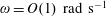
 $$\begin{eqnarray}\displaystyle [\unicode[STIX]{x1D6F7}_{x}]_{x=x^{\pm }} & = & \displaystyle -\unicode[STIX]{x1D6E9}_{t}\frac{z+\unicode[STIX]{x1D707}}{\unicode[STIX]{x1D707}}+\unicode[STIX]{x1D716}\unicode[STIX]{x1D6E9}(z+\unicode[STIX]{x1D707})[\unicode[STIX]{x1D6F7}_{xx}]_{x=x^{\pm }}-\unicode[STIX]{x1D716}^{2}\unicode[STIX]{x1D6E9}^{2}(z+\unicode[STIX]{x1D707})^{2}\left[\frac{\unicode[STIX]{x1D6F7}_{xxx}}{2}\right]_{x=x^{\pm }}\nonumber\\ \displaystyle & & \displaystyle \quad -\,\unicode[STIX]{x1D716}^{2}\unicode[STIX]{x1D6E9}^{2}\unicode[STIX]{x1D6E9}_{t}\frac{z+\unicode[STIX]{x1D707}}{\unicode[STIX]{x1D707}}-\unicode[STIX]{x1D716}\unicode[STIX]{x1D6E9}[\unicode[STIX]{x1D6F7}_{z}^{\pm }]_{x=x^{\pm }}+\unicode[STIX]{x1D716}^{2}\unicode[STIX]{x1D6E9}^{2}(z+\unicode[STIX]{x1D707})[\unicode[STIX]{x1D6F7}_{zx}^{\pm }]_{x=x^{\pm }}\nonumber\\ \displaystyle & & \displaystyle \pm \,\unicode[STIX]{x1D716}\,d\unicode[STIX]{x1D6E9}\unicode[STIX]{x1D6E9}_{t}+O(\unicode[STIX]{x1D716}^{3}),\end{eqnarray}$$
where
 $x^{\pm }=\pm \unicode[STIX]{x1D707}d$
is a new variable. The equation of motion (2.12) becomes
$x^{\pm }=\pm \unicode[STIX]{x1D707}d$
is a new variable. The equation of motion (2.12) becomes
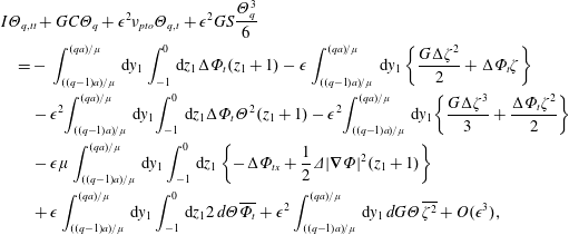 $$\begin{eqnarray}\displaystyle & & \displaystyle I\unicode[STIX]{x1D6E9}_{q,tt}+GC\unicode[STIX]{x1D6E9}_{q}+\unicode[STIX]{x1D716}^{2}\unicode[STIX]{x1D708}_{pto}\unicode[STIX]{x1D6E9}_{q,t}+\unicode[STIX]{x1D716}^{2}GS\frac{\unicode[STIX]{x1D6E9}_{q}^{3}}{6}\nonumber\\ \displaystyle & & \displaystyle \quad =-\,\int _{((q-1)a)/\unicode[STIX]{x1D707}}^{(qa)/\unicode[STIX]{x1D707}}\,\text{d}y_{1}\int _{-1}^{0}\,\text{d}z_{1}\unicode[STIX]{x0394}\unicode[STIX]{x1D6F7}_{t}(z_{1}+1)-\unicode[STIX]{x1D716}\int _{((q-1)a)/\unicode[STIX]{x1D707}}^{(qa)/\unicode[STIX]{x1D707}}\,\text{d}y_{1}\left\{\frac{G\unicode[STIX]{x0394}\unicode[STIX]{x1D701}^{2}}{2}+\unicode[STIX]{x0394}\unicode[STIX]{x1D6F7}_{t}\unicode[STIX]{x1D701}\right\}\nonumber\\ \displaystyle & & \displaystyle \qquad -\,\unicode[STIX]{x1D716}^{2}\!\int _{((q-1)a)/\unicode[STIX]{x1D707}}^{(qa)/\unicode[STIX]{x1D707}}\,\text{d}y_{1}\!\int _{-1}^{0}\,\text{d}z_{1}\unicode[STIX]{x0394}\unicode[STIX]{x1D6F7}_{t}\unicode[STIX]{x1D6E9}^{2}(z_{1}+1)-\unicode[STIX]{x1D716}^{2}\!\int _{((q-1)a)/\unicode[STIX]{x1D707}}^{(qa)/\unicode[STIX]{x1D707}}\,\text{d}y_{1}\!\left\{\frac{G\unicode[STIX]{x0394}\unicode[STIX]{x1D701}^{3}}{3}+\frac{\unicode[STIX]{x0394}\unicode[STIX]{x1D6F7}_{t}\unicode[STIX]{x1D701}^{2}}{2}\right\}\nonumber\\ \displaystyle & & \displaystyle \qquad -\,\unicode[STIX]{x1D716}\unicode[STIX]{x1D707}\int _{((q-1)a)/\unicode[STIX]{x1D707}}^{(qa)/\unicode[STIX]{x1D707}}\,\text{d}y_{1}\int _{-1}^{0}\,\text{d}z_{1}\left\{-\unicode[STIX]{x0394}\unicode[STIX]{x1D6F7}_{tx}+\frac{1}{2}\unicode[STIX]{x1D6E5}|\unicode[STIX]{x1D735}\unicode[STIX]{x1D6F7}|^{2}(z_{1}+1)\right\}\nonumber\\ \displaystyle & & \displaystyle \qquad +\,\unicode[STIX]{x1D716}\int _{((q-1)a)/\unicode[STIX]{x1D707}}^{(qa)/\unicode[STIX]{x1D707}}\,\text{d}y_{1}\int _{-1}^{0}\,\text{d}z_{1}2\,d\unicode[STIX]{x1D6E9}\overline{\unicode[STIX]{x1D6F7}_{t}}+\unicode[STIX]{x1D716}^{2}\int _{((q-1)a)/\unicode[STIX]{x1D707}}^{(qa)/\unicode[STIX]{x1D707}}\,\text{d}y_{1}\,dG\unicode[STIX]{x1D6E9}\overline{\unicode[STIX]{x1D701}^{2}}+O(\unicode[STIX]{x1D716}^{3}),\end{eqnarray}$$
where
 $C=ad/\unicode[STIX]{x1D707}-S$
is the non-dimensional buoyancy restoring torque, while
$C=ad/\unicode[STIX]{x1D707}-S$
is the non-dimensional buoyancy restoring torque, while
 $\unicode[STIX]{x1D6E5}(\cdot )=(\cdot )_{x=x^{+}}^{+}-(\cdot )_{x=x^{-}}^{-}$
and
$\unicode[STIX]{x1D6E5}(\cdot )=(\cdot )_{x=x^{+}}^{+}-(\cdot )_{x=x^{-}}^{-}$
and
 $\overline{(\cdot )}=[(\cdot )_{x=x^{+}}^{+}+(\cdot )_{x=x^{-}}^{-}]/2$
denote respectively the difference and the average of
$\overline{(\cdot )}=[(\cdot )_{x=x^{+}}^{+}+(\cdot )_{x=x^{-}}^{-}]/2$
denote respectively the difference and the average of
 $(\cdot )$
on two sides of the array. A summary of the physical quantities as well as the dimensionless quantities is provided in tables 1 and 2.
$(\cdot )$
on two sides of the array. A summary of the physical quantities as well as the dimensionless quantities is provided in tables 1 and 2.
Table 1. Physical parameters and their dimensions.
Table 2. Dimensionless quantities.

3 Multiple-scale analysis
Let us introduce the following expansions of the non-dimensional velocity potential, free-surface elevation and gate oscillations:
 $$\begin{eqnarray}\displaystyle & \displaystyle \unicode[STIX]{x1D6F7}^{\pm }=\unicode[STIX]{x1D6F7}_{1}^{\pm }(x,y,z,t,t_{2})+\unicode[STIX]{x1D716}\unicode[STIX]{x1D6F7}_{2}^{\pm }(x,y,z,t,t_{2})+\unicode[STIX]{x1D716}^{2}\unicode[STIX]{x1D6F7}_{3}^{\pm }(x,y,z,t,t_{2})+O(\unicode[STIX]{x1D716}^{3}), & \displaystyle\end{eqnarray}$$
 $$\begin{eqnarray}\displaystyle & \displaystyle \unicode[STIX]{x1D701}^{\pm }=\unicode[STIX]{x1D701}_{1}^{\pm }(x,y,t,t_{2})+\unicode[STIX]{x1D716}\unicode[STIX]{x1D701}_{2}^{\pm }(x,y,t,t_{2})+\unicode[STIX]{x1D716}^{2}\unicode[STIX]{x1D701}_{3}^{\pm }(x,y,t,t_{2})+O(\unicode[STIX]{x1D716}^{3}), & \displaystyle\end{eqnarray}$$
 $$\begin{eqnarray}\displaystyle & \displaystyle \unicode[STIX]{x1D6E9}^{\pm }=\unicode[STIX]{x1D6E9}_{1}^{\pm }(y,t,t_{2})+\unicode[STIX]{x1D716}\unicode[STIX]{x1D6E9}_{2}^{\pm }(y,t,t_{2})+\unicode[STIX]{x1D716}^{2}\unicode[STIX]{x1D6E9}_{3}^{\pm }(y,t,t_{2})+O(\unicode[STIX]{x1D716}^{3}), & \displaystyle\end{eqnarray}$$
where
 $t_{2}=\unicode[STIX]{x1D716}^{2}t$
denotes the slow time scale of the modal amplitude growth. Governing equation and boundary conditions yield for
$t_{2}=\unicode[STIX]{x1D716}^{2}t$
denotes the slow time scale of the modal amplitude growth. Governing equation and boundary conditions yield for
 $n=1,2,3,$
the following equations.
$n=1,2,3,$
the following equations.
Laplace equation:
 $$\begin{eqnarray}\unicode[STIX]{x1D6FB}^{2}\unicode[STIX]{x1D6F7}_{n}^{\pm }=0,\quad \text{in }\unicode[STIX]{x1D6FA}^{\pm }.\end{eqnarray}$$
Free-surface dynamic condition:
 $$\begin{eqnarray}-G\unicode[STIX]{x1D701}_{n}^{\pm }={\mathcal{B}}_{n},\quad z=0,\end{eqnarray}$$
where
 $$\begin{eqnarray}\displaystyle & \displaystyle {\mathcal{B}}_{1}=\unicode[STIX]{x1D6F7}_{1_{t}}^{\pm }, & \displaystyle\end{eqnarray}$$
 $$\begin{eqnarray}\displaystyle & \displaystyle {\mathcal{B}}_{2}=\unicode[STIX]{x1D6F7}_{2_{t}}^{\pm }, & \displaystyle\end{eqnarray}$$
 $$\begin{eqnarray}\displaystyle & \displaystyle {\mathcal{B}}_{3}=\unicode[STIX]{x1D6F7}_{3_{t}}^{\pm }+\unicode[STIX]{x1D6F7}_{1_{tz}}^{\pm }\unicode[STIX]{x1D701}_{1}^{\pm }+{\textstyle \frac{1}{2}}|\unicode[STIX]{x1D735}\unicode[STIX]{x1D6F7}_{1}^{\pm }|^{2}+\unicode[STIX]{x1D6F7}_{1_{t_{2}}}^{\pm }. & \displaystyle\end{eqnarray}$$
Free-surface mixed condition:
 $$\begin{eqnarray}\unicode[STIX]{x1D6F7}_{n_{tt}}^{\pm }+G\unicode[STIX]{x1D6F7}_{n_{z}}={\mathcal{F}}_{n},\quad z=0,\end{eqnarray}$$
where
 $$\begin{eqnarray}\displaystyle & \displaystyle {\mathcal{F}}_{1}=0, & \displaystyle\end{eqnarray}$$
 $$\begin{eqnarray}\displaystyle & \displaystyle {\mathcal{F}}_{2}=0, & \displaystyle\end{eqnarray}$$
 $$\begin{eqnarray}\displaystyle & \displaystyle {\mathcal{F}}_{3}=-(\unicode[STIX]{x1D6F7}_{1_{ttz}}^{\pm }+G\unicode[STIX]{x1D6F7}_{1_{zz}}^{\pm })\unicode[STIX]{x1D701}_{1}^{\pm }-|\unicode[STIX]{x1D735}\unicode[STIX]{x1D6F7}_{1_{t}}^{\pm }|^{2}-2\unicode[STIX]{x1D6F7}_{1_{tt_{2}}}^{\pm }. & \displaystyle\end{eqnarray}$$
No-flux boundary condition at the bottom:
 $$\begin{eqnarray}\unicode[STIX]{x1D6F7}_{n_{z}}=0,\quad z=-h.\end{eqnarray}$$
No-flux boundary condition on the channel walls:
 $$\begin{eqnarray}\unicode[STIX]{x1D6F7}_{n_{y}}=0,\quad y=0\quad \text{and}\quad y=b.\end{eqnarray}$$
Kinematic condition on the array surface:
 $$\begin{eqnarray}\unicode[STIX]{x1D6F7}_{n_{x}}=\left(-\unicode[STIX]{x1D6E9}_{n_{t}}\frac{z+\unicode[STIX]{x1D707}}{\unicode[STIX]{x1D707}}+{\mathcal{G}}_{n}\right)H(z+h-c),\quad x=x^{\pm },\end{eqnarray}$$
where
 $$\begin{eqnarray}\displaystyle & \displaystyle {\mathcal{G}}_{1}=0, & \displaystyle\end{eqnarray}$$
 $$\begin{eqnarray}\displaystyle & \displaystyle {\mathcal{G}}_{2}=-\unicode[STIX]{x1D6F7}_{1_{z}}^{\pm }\unicode[STIX]{x1D6E9}_{1}\pm \,d\unicode[STIX]{x1D6E9}_{1}\unicode[STIX]{x1D6E9}_{1_{t}}, & \displaystyle\end{eqnarray}$$
 $$\begin{eqnarray}\displaystyle {\mathcal{G}}_{3} & = & \displaystyle \unicode[STIX]{x1D6F7}_{1_{xx}}^{\pm }\unicode[STIX]{x1D6E9}_{1}(z+\unicode[STIX]{x1D707})-\unicode[STIX]{x1D6E9}_{1_{t}}\unicode[STIX]{x1D6E9}_{1}^{2}\frac{z+\unicode[STIX]{x1D707}}{\unicode[STIX]{x1D707}}-\unicode[STIX]{x1D6F7}_{2_{z}}^{\pm }\unicode[STIX]{x1D6E9}_{1}-\unicode[STIX]{x1D6F7}_{1_{z}}^{\pm }\unicode[STIX]{x1D6E9}_{2}\nonumber\\ \displaystyle & & \displaystyle -\,\unicode[STIX]{x1D6E9}_{1_{t_{2}}}\frac{z+\unicode[STIX]{x1D707}}{\unicode[STIX]{x1D707}}\pm \,d(\unicode[STIX]{x1D6E9}_{1}\unicode[STIX]{x1D6E9}_{2})_{t}.\end{eqnarray}$$
Equation of motion of the
 $q$
th gate:
$q$
th gate:
 $$\begin{eqnarray}I\unicode[STIX]{x1D6E9}_{q,n_{tt}}+GC\unicode[STIX]{x1D6E9}_{q,n}=-\int _{((q-1)a)/\unicode[STIX]{x1D707}}^{(qa)/\unicode[STIX]{x1D707}}\,\text{d}y_{1}\int _{-1}^{0}\,\text{d}z_{1}\unicode[STIX]{x0394}\unicode[STIX]{x1D6F7}_{n_{t}}^{\pm }(z_{1}+1)+{\mathcal{D}}_{n},\end{eqnarray}$$
where
 $$\begin{eqnarray}\displaystyle & \displaystyle {\mathcal{D}}_{1}=0, & \displaystyle\end{eqnarray}$$
 $$\begin{eqnarray}\displaystyle & \displaystyle {\mathcal{D}}_{2}=-\int _{((q-1)a)/\unicode[STIX]{x1D707}}^{(qa)/\unicode[STIX]{x1D707}}\,\text{d}y_{1}\left\{G\frac{\unicode[STIX]{x0394}\unicode[STIX]{x1D701}_{1}^{2}}{2}+\unicode[STIX]{x0394}\unicode[STIX]{x1D6F7}_{1_{t}}\unicode[STIX]{x1D701}_{1}\right\}+\int _{((q-1)a)/\unicode[STIX]{x1D707}}^{(qa)/\unicode[STIX]{x1D707}}\,\text{d}y_{1}\int _{-1}^{0}\,\text{d}z_{1}2d\unicode[STIX]{x1D6E9}_{1}\overline{\unicode[STIX]{x1D6F7}_{1_{t}}},\qquad & \displaystyle\end{eqnarray}$$
 $$\begin{eqnarray}\displaystyle {\mathcal{D}}_{3} & = & \displaystyle -\int _{((q-1)a)/\unicode[STIX]{x1D707}}^{(qa)/\unicode[STIX]{x1D707}}\,\text{d}y_{1}\int _{-1}^{0}\,\text{d}z_{1}\left\{\left[\unicode[STIX]{x0394}\unicode[STIX]{x1D6F7}_{1_{t}}\unicode[STIX]{x1D6E9}_{1}^{2}-\frac{\unicode[STIX]{x1D707}}{\unicode[STIX]{x1D716}}\unicode[STIX]{x0394}\unicode[STIX]{x1D6F7}_{1_{tx}}\unicode[STIX]{x1D6E9}_{2}(z_{1}+1)+\frac{\unicode[STIX]{x1D707}}{\unicode[STIX]{x1D716}}\frac{1}{2}\unicode[STIX]{x1D6E5}|\unicode[STIX]{x1D735}\unicode[STIX]{x1D6F7}_{1}|^{2}\right.\right.\nonumber\\ \displaystyle & & \displaystyle +\left.\left.\,\unicode[STIX]{x0394}\unicode[STIX]{x1D6F7}_{1_{t_{2}}}\right](z_{1}+1)\right\}-\int _{((q-1)a)/\unicode[STIX]{x1D707}}^{(qa)/\unicode[STIX]{x1D707}}\,\text{d}y_{1}\left\{G\frac{\unicode[STIX]{x0394}\unicode[STIX]{x1D701}^{3}}{3}+\frac{\unicode[STIX]{x0394}\unicode[STIX]{x1D6F7}_{1_{t}}\unicode[STIX]{x1D701}_{1}^{2}}{2}+G\unicode[STIX]{x0394}\unicode[STIX]{x1D701}_{1}\unicode[STIX]{x1D701}_{2}+\unicode[STIX]{x0394}\unicode[STIX]{x1D6F7}_{1_{t}}\unicode[STIX]{x1D701}_{2}\right.\nonumber\\ \displaystyle & & \displaystyle +\left.\,\unicode[STIX]{x0394}\unicode[STIX]{x1D6F7}_{2_{t}}\unicode[STIX]{x1D701}_{1}\right\}-\unicode[STIX]{x1D708}_{pto}\unicode[STIX]{x1D6E9}_{q,1_{t}}-2I\unicode[STIX]{x1D6E9}_{q,1_{tt_{2}}}+\int _{((q-1)a)/\unicode[STIX]{x1D707}}^{(qa)/\unicode[STIX]{x1D707}}\,\text{d}y_{1}\int _{-1}^{0}\,\text{d}z_{1}2\,d\{\unicode[STIX]{x1D6E9}_{1}\overline{\unicode[STIX]{x1D6F7}_{2_{t}}}+\unicode[STIX]{x1D6E9}_{2}\overline{\unicode[STIX]{x1D6F7}_{1_{t}}}\}\nonumber\\ \displaystyle & & \displaystyle \times \,\int _{((q-1)a)/\unicode[STIX]{x1D707}}^{(qa)/\unicode[STIX]{x1D707}}\,\text{d}y_{1}\,dG\unicode[STIX]{x1D6E9}_{1}\overline{\unicode[STIX]{x1D701}_{1}^{2}}-\frac{GS}{6}\unicode[STIX]{x1D6E9}_{q,1}^{3}.\end{eqnarray}$$
The latter forcing terms are algebraically simpler than those of Sammarco et al. (Reference Sammarco, Tran and Mei1997a
). Indeed, the second-order boundary problem of Sammarco et al. (Reference Sammarco, Tran and Mei1997a
) is forced on the free surface by the first-order solution. In the present case instead, the forcing term for the second-order free-surface mixed boundary condition
 ${\mathcal{F}}_{2}$
is null, as well as
${\mathcal{F}}_{2}$
is null, as well as
 ${\mathcal{F}}_{1}$
. This simplifies considerably the required algebra to seek the second-order solution because now the boundary conditions at
${\mathcal{F}}_{1}$
. This simplifies considerably the required algebra to seek the second-order solution because now the boundary conditions at
 $z=0$
and
$z=0$
and
 $z=-h$
are homogeneous and similar to those for the leading-order problem
$z=-h$
are homogeneous and similar to those for the leading-order problem
 $O(1)$
. Nevertheless, the dominant nonlinear effects are given by
$O(1)$
. Nevertheless, the dominant nonlinear effects are given by
 ${\mathcal{G}}_{2}$
(3.17) and
${\mathcal{G}}_{2}$
(3.17) and
 ${\mathcal{D}}_{2}$
(3.21).
${\mathcal{D}}_{2}$
(3.21).
4 Subharmonic excitation of a single mode
It is known that an incident wave of frequency
 $2\unicode[STIX]{x1D714}$
and amplitude
$2\unicode[STIX]{x1D714}$
and amplitude
 $O(\unicode[STIX]{x1D716})$
excites subharmonically a trapped mode of frequency
$O(\unicode[STIX]{x1D716})$
excites subharmonically a trapped mode of frequency
 $\unicode[STIX]{x1D714}$
of an array of floating gates (Mei et al.
Reference Mei, Sammarco, Chan and Procaccini1994; Sammarco et al.
Reference Sammarco, Tran and Mei1997a
,Reference Sammarco, Tran, Gottlieb and Mei
b
). A similar resonance mechanism is known in the context of edge waves. In this section we analyse the subharmonic resonance of a single trapped natural mode of an array of
$\unicode[STIX]{x1D714}$
of an array of floating gates (Mei et al.
Reference Mei, Sammarco, Chan and Procaccini1994; Sammarco et al.
Reference Sammarco, Tran and Mei1997a
,Reference Sammarco, Tran, Gottlieb and Mei
b
). A similar resonance mechanism is known in the context of edge waves. In this section we analyse the subharmonic resonance of a single trapped natural mode of an array of
 $Q$
gates. Performing harmonic expansion of the governing equations, we obtain that the zeroth harmonic problem at the first and second order is unforced while the boundary value problem governing the first harmonic at the second order is identical to that governing the first harmonic at the first order (Sammarco et al.
Reference Sammarco, Tran and Mei1997a
). For these reasons, we return in physical variables, omit the primes for brevity and assume the following solution:
$Q$
gates. Performing harmonic expansion of the governing equations, we obtain that the zeroth harmonic problem at the first and second order is unforced while the boundary value problem governing the first harmonic at the second order is identical to that governing the first harmonic at the first order (Sammarco et al.
Reference Sammarco, Tran and Mei1997a
). For these reasons, we return in physical variables, omit the primes for brevity and assume the following solution:
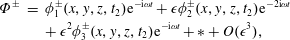 $$\begin{eqnarray}\displaystyle \unicode[STIX]{x1D6F7}^{\pm } & = & \displaystyle \unicode[STIX]{x1D719}_{1}^{\pm }(x,y,z,t_{2})\text{e}^{-\text{i}\unicode[STIX]{x1D714}t}+\unicode[STIX]{x1D716}\unicode[STIX]{x1D719}_{2}^{\pm }(x,y,z,t_{2})\text{e}^{-2\text{i}\unicode[STIX]{x1D714}t}\nonumber\\ \displaystyle & & \displaystyle +\,\unicode[STIX]{x1D716}^{2}\unicode[STIX]{x1D719}_{3}^{\pm }(x,y,z,t_{2})\text{e}^{-\text{i}\unicode[STIX]{x1D714}t}+\ast +O(\unicode[STIX]{x1D716}^{3}),\end{eqnarray}$$
 $$\begin{eqnarray}\displaystyle & \displaystyle \unicode[STIX]{x1D701}^{\pm }=\unicode[STIX]{x1D702}_{1}^{\pm }(x,y,t_{2})\text{e}^{-\text{i}\unicode[STIX]{x1D714}t}+\unicode[STIX]{x1D716}\unicode[STIX]{x1D702}_{2}^{\pm }(x,y,t_{2})\text{e}^{-2\text{i}\unicode[STIX]{x1D714}t}+\unicode[STIX]{x1D716}^{2}\unicode[STIX]{x1D702}_{3}^{\pm }(x,y,t_{2})\text{e}^{-\text{i}\unicode[STIX]{x1D714}t}+\ast +O(\unicode[STIX]{x1D716}^{3}), & \displaystyle\end{eqnarray}$$
 $$\begin{eqnarray}\displaystyle & \displaystyle \unicode[STIX]{x1D6E9}=\unicode[STIX]{x1D703}_{1}(y,t_{2})\text{e}^{-\text{i}\unicode[STIX]{x1D714}t}+\unicode[STIX]{x1D716}\unicode[STIX]{x1D703}_{2}(y,t_{2})\text{e}^{-2\text{i}\unicode[STIX]{x1D714}t}+\unicode[STIX]{x1D716}^{2}\unicode[STIX]{x1D703}_{3}(y,t_{2})\text{e}^{-\text{i}\unicode[STIX]{x1D714}t}+\ast +O(\unicode[STIX]{x1D716}^{3}), & \displaystyle\end{eqnarray}$$
where
 $\ast$
denotes the complex conjugate and the second-order problem includes the harmonic
$\ast$
denotes the complex conjugate and the second-order problem includes the harmonic
 $2\unicode[STIX]{x1D714}$
only.
$2\unicode[STIX]{x1D714}$
only.
4.1 Leading-order problem
 $O(1)$

The
 $O(1)$
problem is homogeneous and unforced. Solution of the governing equations yields the well-known trapped natural modes of an array of
$O(1)$
problem is homogeneous and unforced. Solution of the governing equations yields the well-known trapped natural modes of an array of
 $Q$
gates in an infinitely long channel (Mei et al.
Reference Mei, Sammarco, Chan and Procaccini1994; Li & Mei Reference Li and Mei2003; Sammarco et al.
Reference Sammarco, Michele and d’Errico2013). The boundary value problem at the leading order is governed by the following equations:
$Q$
gates in an infinitely long channel (Mei et al.
Reference Mei, Sammarco, Chan and Procaccini1994; Li & Mei Reference Li and Mei2003; Sammarco et al.
Reference Sammarco, Michele and d’Errico2013). The boundary value problem at the leading order is governed by the following equations:
 $$\begin{eqnarray}\unicode[STIX]{x1D6FB}^{2}\unicode[STIX]{x1D719}_{1}^{\pm }=0,\quad \text{in }\unicode[STIX]{x1D6FA}^{\pm }\end{eqnarray}$$
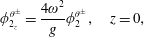
 $$\begin{eqnarray}\unicode[STIX]{x1D719}_{1_{z}}^{\pm }=\unicode[STIX]{x1D719}_{1}^{\pm }\frac{\unicode[STIX]{x1D714}^{2}}{g},\quad z=0,\end{eqnarray}$$
 $$\begin{eqnarray}\unicode[STIX]{x1D702}_{1}^{\pm }=\frac{\text{i}\unicode[STIX]{x1D714}}{g}\unicode[STIX]{x1D719}_{1}^{\pm },\quad z=0,\end{eqnarray}$$
 $$\begin{eqnarray}\unicode[STIX]{x1D719}_{1_{x}}^{\pm }=\text{i}\unicode[STIX]{x1D714}\unicode[STIX]{x1D703}_{1}(z+h_{p})H(z+h-c),\quad x=x^{\pm }.\end{eqnarray}$$
By defining
 $\unicode[STIX]{x1D703}_{1}=\{r_{1q}\}\unicode[STIX]{x1D703}(t_{2})$
, with
$\unicode[STIX]{x1D703}_{1}=\{r_{1q}\}\unicode[STIX]{x1D703}(t_{2})$
, with
 $\{r_{1q}\}=\{r_{11},\ldots ,r_{1Q}\}$
the modal shape, we obtain the solution of the velocity potential,
$\{r_{1q}\}=\{r_{11},\ldots ,r_{1Q}\}$
the modal shape, we obtain the solution of the velocity potential,
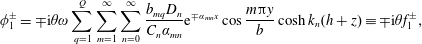 $$\begin{eqnarray}\unicode[STIX]{x1D719}_{1}^{\pm }=\mp \text{i}\unicode[STIX]{x1D703}\unicode[STIX]{x1D714}\mathop{\sum }_{q=1}^{Q}\mathop{\sum }_{m=1}^{\infty }\mathop{\sum }_{n=0}^{\infty }\frac{b_{mq}D_{n}}{C_{n}\unicode[STIX]{x1D6FC}_{mn}}\text{e}^{\mp \unicode[STIX]{x1D6FC}_{mn}x}\cos \frac{m\unicode[STIX]{x03C0}y}{b}\cosh k_{n}(h+z)\equiv \mp \text{i}\unicode[STIX]{x1D703}f_{1}^{\pm },\end{eqnarray}$$
and of the free-surface elevation,
 $$\begin{eqnarray}\unicode[STIX]{x1D702}_{1}^{\pm }=\pm \frac{\unicode[STIX]{x1D714}}{g}f_{1}^{\pm }\unicode[STIX]{x1D703},\end{eqnarray}$$
with
 $k_{n}$
being the roots of the dispersion relation
$k_{n}$
being the roots of the dispersion relation
 $$\begin{eqnarray}\left.\begin{array}{@{}c@{}}\displaystyle \unicode[STIX]{x1D714}^{2}=gk_{0}\tanh k_{0}h,\\ \unicode[STIX]{x1D714}^{2}=-g\overline{k}_{n}\tan \overline{k}_{n}h,\quad k_{n}=\text{i}\overline{k}_{n},n=1,\ldots ,\infty .\end{array}\right\}\end{eqnarray}$$
The real coefficients
 $b_{mq}$
,
$b_{mq}$
,
 $\unicode[STIX]{x1D6FC}_{mn}$
,
$\unicode[STIX]{x1D6FC}_{mn}$
,
 $C_{n}$
and
$C_{n}$
and
 $D_{n}$
are defined by
$D_{n}$
are defined by
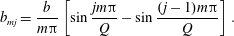
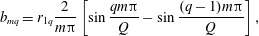 $$\begin{eqnarray}\displaystyle & \displaystyle b_{mq}=r_{1q}\frac{2}{m\unicode[STIX]{x03C0}}\left[\sin \frac{qm\unicode[STIX]{x03C0}}{Q}-\sin \frac{(q-1)m\unicode[STIX]{x03C0}}{Q}\right], & \displaystyle\end{eqnarray}$$
 $$\begin{eqnarray}\displaystyle & \displaystyle \unicode[STIX]{x1D6FC}_{mn}=\sqrt{\left(\frac{m\unicode[STIX]{x03C0}}{b}\right)^{2}-k_{n}^{2}}, & \displaystyle\end{eqnarray}$$
 $$\begin{eqnarray}\displaystyle & \displaystyle C_{n}=\frac{1}{2}\left(h+\frac{g}{\unicode[STIX]{x1D714}^{2}}\sinh ^{2}k_{n}h\right), & \displaystyle\end{eqnarray}$$
 $$\begin{eqnarray}\displaystyle & \displaystyle D_{n}=\frac{1}{k_{n}^{2}}[\cosh k_{n}c-\cosh k_{n}h+k_{n}(h-c)\sinh k_{n}h]. & \displaystyle\end{eqnarray}$$
Note that the real function
 $f_{1}^{\pm }$
defined in (4.8) has the properties
$f_{1}^{\pm }$
defined in (4.8) has the properties
 $$\begin{eqnarray}f_{1}^{+}(x)=f_{1}^{-}(-x),\quad f_{1_{x}}^{+}(x)=-f_{1_{x}}^{-}(-x),\end{eqnarray}$$
and that the wavenumber
 $k_{0}$
must satisfy the condition
$k_{0}$
must satisfy the condition
 $k_{0}<\unicode[STIX]{x03C0}/b$
in order that the absence/existence of propagating waves/trapped modes is satisfied.
$k_{0}<\unicode[STIX]{x03C0}/b$
in order that the absence/existence of propagating waves/trapped modes is satisfied.
Conservation of angular momentum for each gate
 $G_{j}$
requires that
$G_{j}$
requires that
 $$\begin{eqnarray}r_{1j}(-\unicode[STIX]{x1D714}^{2}I+C)-\unicode[STIX]{x1D714}^{2}I_{j}=0,\end{eqnarray}$$
where
 $I_{j}$
is the added inertia defined as
$I_{j}$
is the added inertia defined as
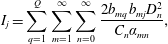 $$\begin{eqnarray}I_{j}=\mathop{\sum }_{q=1}^{Q}\mathop{\sum }_{m=1}^{\infty }\mathop{\sum }_{n=0}^{\infty }\frac{2b_{mq}b_{mj}D_{n}^{2}}{C_{n}\unicode[STIX]{x1D6FC}_{mn}},\end{eqnarray}$$
with
 $$\begin{eqnarray}b_{mj}=\frac{b}{m\unicode[STIX]{x03C0}}\left[\sin \frac{jm\unicode[STIX]{x03C0}}{Q}-\sin \frac{(j-1)m\unicode[STIX]{x03C0}}{Q}\right].\end{eqnarray}$$
As in Sammarco et al. (Reference Sammarco, Michele and d’Errico2013), solution of (4.16) yields
 $(Q-1)$
out-of-phase natural modes and related eigenfrequencies. The reader should refer to the work of Li & Mei (Reference Li and Mei2003) for a complete list of modal shapes in which
$(Q-1)$
out-of-phase natural modes and related eigenfrequencies. The reader should refer to the work of Li & Mei (Reference Li and Mei2003) for a complete list of modal shapes in which
 $2\leqslant Q\leqslant 20$
.
$2\leqslant Q\leqslant 20$
.
4.2 The second-order problem
$O(\unicode[STIX]{x1D716})$

Since the incident wave field is assumed to be at
 $O(\unicode[STIX]{x1D716})$
, the incident wave amplitude
$O(\unicode[STIX]{x1D716})$
, the incident wave amplitude
 $A^{\prime }$
must be an order smaller than
$A^{\prime }$
must be an order smaller than
 $A_{T}^{\prime }$
, thus
$A_{T}^{\prime }$
, thus
 $A^{\prime }/A_{T}^{\prime }=O(\unicode[STIX]{x1D716})$
. Hence, at
$A^{\prime }/A_{T}^{\prime }=O(\unicode[STIX]{x1D716})$
. Hence, at
 $O(\unicode[STIX]{x1D716})$
we assume the coexistence of the second harmonic
$O(\unicode[STIX]{x1D716})$
we assume the coexistence of the second harmonic
 $2\unicode[STIX]{x1D714}$
with two components:
$2\unicode[STIX]{x1D714}$
with two components:
 $$\begin{eqnarray}\unicode[STIX]{x1D719}_{2}^{\pm }=\unicode[STIX]{x1D719}_{2}^{\unicode[STIX]{x1D703}^{\pm }}+\unicode[STIX]{x1D719}^{A^{\pm }},\end{eqnarray}$$
where
 $\unicode[STIX]{x1D719}_{2}^{\unicode[STIX]{x1D703}^{\pm }}$
is the second-order potential forced by the quadratic products (3.17) on the gate surface, while
$\unicode[STIX]{x1D719}_{2}^{\unicode[STIX]{x1D703}^{\pm }}$
is the second-order potential forced by the quadratic products (3.17) on the gate surface, while
 $\unicode[STIX]{x1D719}^{A^{\pm }}$
is the second-order potential forced by the incident wave field.
$\unicode[STIX]{x1D719}^{A^{\pm }}$
is the second-order potential forced by the incident wave field.
4.2.1 Radiated second harmonic –
$\unicode[STIX]{x1D719}_{2}^{\unicode[STIX]{x1D703}^{\pm }}$

The kinematic condition on the moving gates includes a forcing term,
 $$\begin{eqnarray}\unicode[STIX]{x1D719}_{2_{x}}^{\unicode[STIX]{x1D703}^{\pm }}=\left[2\text{i}\unicode[STIX]{x1D714}\unicode[STIX]{x1D703}_{2}^{\unicode[STIX]{x1D703}}(z+h_{p})-\frac{\unicode[STIX]{x1D719}_{1_{z}}^{\pm }\unicode[STIX]{x1D703}_{1}}{\unicode[STIX]{x1D716}}\mp \text{i}\unicode[STIX]{x1D714}\,d\frac{\unicode[STIX]{x1D703}_{1}^{2}}{\unicode[STIX]{x1D716}}\right]H(z+h-c),\quad x=x^{\pm },\end{eqnarray}$$
while the governing equation and the remaining boundary conditions on the free surface remain homogeneous like the
 $O(1)$
problem:
$O(1)$
problem:
 $$\begin{eqnarray}\unicode[STIX]{x1D6FB}^{2}\unicode[STIX]{x1D719}_{2}^{\unicode[STIX]{x1D703}^{\pm }}=0,\end{eqnarray}$$
 $$\begin{eqnarray}\unicode[STIX]{x1D719}_{2_{z}}^{\unicode[STIX]{x1D703}^{\pm }}=\frac{4\unicode[STIX]{x1D714}^{2}}{g}\unicode[STIX]{x1D719}_{2}^{\unicode[STIX]{x1D703}^{\pm }},\quad z=0,\end{eqnarray}$$
 $$\begin{eqnarray}\unicode[STIX]{x1D702}_{2}^{\unicode[STIX]{x1D703}^{\pm }}=\frac{2\text{i}\unicode[STIX]{x1D714}}{g}\unicode[STIX]{x1D719}_{2}^{\unicode[STIX]{x1D703}^{\pm }},\quad z=0.\end{eqnarray}$$
As the forcing term in (4.20) contains only the second harmonic, we assume the solution of the potential
 $\unicode[STIX]{x1D719}_{2}^{\unicode[STIX]{x1D703}^{\pm }}$
and of the angular motion
$\unicode[STIX]{x1D719}_{2}^{\unicode[STIX]{x1D703}^{\pm }}$
and of the angular motion
 $\unicode[STIX]{x1D703}_{2}$
in the form
$\unicode[STIX]{x1D703}_{2}$
in the form
 $$\begin{eqnarray}\unicode[STIX]{x1D719}_{2}^{\unicode[STIX]{x1D703}^{\pm }}=\text{i}\unicode[STIX]{x1D703}^{2}f_{2}^{\pm },\quad \unicode[STIX]{x1D703}_{2}^{\unicode[STIX]{x1D703}}=\text{i}\unicode[STIX]{x1D703}^{2}\unicode[STIX]{x1D703}_{2}.\end{eqnarray}$$
We get the following boundary value problem for the complex function
 $f_{2}^{\pm }$
:
$f_{2}^{\pm }$
:
 $$\begin{eqnarray}\unicode[STIX]{x1D6FB}^{2}f_{2}^{\pm }=0,\end{eqnarray}$$
 $$\begin{eqnarray}f_{2_{z}}^{\pm }=\frac{4\unicode[STIX]{x1D714}^{2}}{g}f_{2}^{\pm },\quad z=0,\end{eqnarray}$$
 $$\begin{eqnarray}f_{2_{x}}^{\pm }=2\text{i}\unicode[STIX]{x1D714}\unicode[STIX]{x1D703}_{2}(z+h_{p})H(z+h-c)\pm \frac{1}{\unicode[STIX]{x1D716}}\mathop{\sum }_{p=0}^{\infty }\unicode[STIX]{x1D6E5}_{p}^{\pm }\cos \frac{p\unicode[STIX]{x03C0}y}{b},\quad x=x^{\pm },\end{eqnarray}$$
where
 $$\begin{eqnarray}\displaystyle \unicode[STIX]{x1D6E5}_{p}^{\pm } & = & \displaystyle \frac{\unicode[STIX]{x1D6FF}_{p}}{b}\int _{0}^{b}\,\text{d}y(f_{1_{z}}^{\pm }r_{1q}-d\unicode[STIX]{x1D714}r_{1q}^{2})\cos \frac{p\unicode[STIX]{x03C0}y}{b}\nonumber\\ \displaystyle & = & \displaystyle \frac{1}{2\unicode[STIX]{x1D6FF}_{p}}\mathop{\sum }_{q=1}^{Q}\left\{\mathop{\sum }_{m=1}^{\infty }b_{(m+p)q}\left[-d\unicode[STIX]{x1D714}b_{mq}+\mathop{\sum }_{n=0}^{\infty }\frac{\unicode[STIX]{x1D714}b_{mq}D_{n}}{C_{n}\unicode[STIX]{x1D6FC}_{mn}}k_{n}\sinh k_{n}(h+z)\right]\right.\nonumber\\ \displaystyle & & \displaystyle \left.+\,\mathop{\sum }_{m=1}^{\infty }b_{mq}\left[-d\unicode[STIX]{x1D714}b_{(m+p)q}+\mathop{\sum }_{n=0}^{\infty }\frac{\unicode[STIX]{x1D714}b_{(m+p)q}D_{n}}{C_{n}\unicode[STIX]{x1D6FC}_{(m+p)n}}k_{n}\sinh k_{n}(h+z)\right]\right\}.\end{eqnarray}$$
Here
 $\unicode[STIX]{x1D6FF}_{p}$
denotes the Jacobi symbol, i.e.
$\unicode[STIX]{x1D6FF}_{p}$
denotes the Jacobi symbol, i.e.
 $\unicode[STIX]{x1D6FF}_{0}=1$
and
$\unicode[STIX]{x1D6FF}_{0}=1$
and
 $\unicode[STIX]{x1D6FF}_{p}=2,p=1,\ldots .$
Note that the latter term is the same in both fluid regions:
$\unicode[STIX]{x1D6FF}_{p}=2,p=1,\ldots .$
Note that the latter term is the same in both fluid regions:
 $\unicode[STIX]{x1D6E5}_{p}^{+}\equiv \unicode[STIX]{x1D6E5}_{p}^{-}$
.
$\unicode[STIX]{x1D6E5}_{p}^{+}\equiv \unicode[STIX]{x1D6E5}_{p}^{-}$
.
Solution of the problem can be found by separation of variables:
 $$\begin{eqnarray}f_{2}^{\pm }=-\text{i}\mathop{\sum }_{p=0}^{\infty }\mathop{\sum }_{l=0}^{\infty }\frac{1}{\unicode[STIX]{x1D6FC}_{pl}}\left(\frac{\unicode[STIX]{x1D6E5}_{pl}}{\unicode[STIX]{x1D716}}\pm \mathop{\sum }_{q=1}^{Q}\frac{2\text{i}b_{pq}\unicode[STIX]{x1D714}D_{l}}{C_{l}}\right)\text{e}^{\pm \text{i}\unicode[STIX]{x1D6FC}_{pl}x}\cos \frac{p\unicode[STIX]{x03C0}y}{b}\cosh \unicode[STIX]{x1D705}_{l}(h+z),\end{eqnarray}$$
where
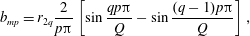 $$\begin{eqnarray}b_{mp}=r_{2q}\frac{2}{p\unicode[STIX]{x03C0}}\left[\sin \frac{qp\unicode[STIX]{x03C0}}{Q}-\sin \frac{(q-1)p\unicode[STIX]{x03C0}}{Q}\right],\end{eqnarray}$$
 $\unicode[STIX]{x1D705}_{l}$
are the real roots of the dispersion relation
$\unicode[STIX]{x1D705}_{l}$
are the real roots of the dispersion relation
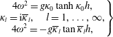 $$\begin{eqnarray}\left.\begin{array}{@{}c@{}}4\unicode[STIX]{x1D714}^{2}=g\unicode[STIX]{x1D705}_{0}\tanh \unicode[STIX]{x1D705}_{0}h,\\ \unicode[STIX]{x1D705}_{l}=\text{i}\overline{\unicode[STIX]{x1D705}}_{l},\quad l=1,\ldots ,\infty ,\\ 4\unicode[STIX]{x1D714}^{2}=-g\overline{\unicode[STIX]{x1D705}}_{l}\tan \overline{\unicode[STIX]{x1D705}}_{l}h,\end{array}\right\}\end{eqnarray}$$
while the coefficient
 $\unicode[STIX]{x1D6E5}_{pl}$
is given by
$\unicode[STIX]{x1D6E5}_{pl}$
is given by
 $$\begin{eqnarray}\displaystyle \unicode[STIX]{x1D6E5}_{pl} & = & \displaystyle \frac{1}{C_{l}}\int _{-h}^{0}\,\text{d}z\unicode[STIX]{x1D6E5}_{p}\cosh \unicode[STIX]{x1D705}_{l}(h+z)\nonumber\\ \displaystyle & = & \displaystyle \frac{1}{2\unicode[STIX]{x1D6FF}_{p}C_{l}}\mathop{\sum }_{q=1}^{Q}\mathop{\sum }_{m=1}^{\infty }\mathop{\sum }_{n=0}^{\infty }\left\{b_{(m+p)q}\left[-d\unicode[STIX]{x1D714}b_{mq}E_{l}+\frac{\unicode[STIX]{x1D714}b_{mq}D_{n}C_{ln}}{C_{n}\unicode[STIX]{x1D6FC}_{mn}}\right]\right.\nonumber\\ \displaystyle & & \displaystyle \left.+\,b_{mq}\left[-d\unicode[STIX]{x1D714}b_{(m+p)q}E_{l}+\frac{\unicode[STIX]{x1D714}b_{(m+p)q}D_{n}C_{ln}}{C_{n}\unicode[STIX]{x1D6FC}_{(m+p)n}}\right]\right\},\end{eqnarray}$$
in which
 $$\begin{eqnarray}\displaystyle C_{ln} & = & \displaystyle \frac{1}{\unicode[STIX]{x1D705}_{l}^{2}-k_{n}^{2}}\left[\cosh k_{n}h\cosh \unicode[STIX]{x1D705}_{l}h\left(\frac{4\unicode[STIX]{x1D714}^{2}}{g^{2}}-k_{n}^{2}\right)\right.\nonumber\\ \displaystyle & & \displaystyle \left.+\,k_{n}^{2}\cosh k_{n}c\cosh \unicode[STIX]{x1D705}_{l}c-\unicode[STIX]{x1D705}_{l}k_{n}\sinh k_{n}h\sinh \unicode[STIX]{x1D705}_{l}h\right],\end{eqnarray}$$
 $$\begin{eqnarray}E_{l}=\frac{1}{\unicode[STIX]{x1D705}_{l}}(\sinh \unicode[STIX]{x1D705}_{l}h-\sinh \unicode[STIX]{x1D705}_{l}c).\end{eqnarray}$$
Because of the symmetry properties (4.15), the equation of motion reads
 $$\begin{eqnarray}r_{2j}(-4\unicode[STIX]{x1D714}^{2}I+C)=2\text{i}\unicode[STIX]{x1D70C}\unicode[STIX]{x1D714}\int _{(j-1)a}^{ja}\,\text{d}y\int _{-h_{p}}^{0}\text{i}\unicode[STIX]{x1D703}\unicode[STIX]{x0394}f_{2}(z+h_{p})\,\text{d}z,\end{eqnarray}$$
however,
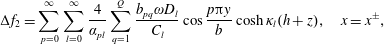 $$\begin{eqnarray}\unicode[STIX]{x0394}f_{2}=\mathop{\sum }_{p=0}^{\infty }\mathop{\sum }_{l=0}^{\infty }\frac{4}{\unicode[STIX]{x1D6FC}_{pl}}\mathop{\sum }_{q=1}^{Q}\frac{b_{pq}\unicode[STIX]{x1D714}D_{l}}{C_{l}}\cos \frac{p\unicode[STIX]{x03C0}y}{b}\cosh \unicode[STIX]{x1D705}_{l}(h+z),\quad x=x^{\pm },\end{eqnarray}$$
so that substitution of the above expression in (4.35) yields a system of homogeneous equations in
 $r_{2j}$
,
$r_{2j}$
,
 $j=1,2$
, with non-zero determinant of the coefficient matrix. As a result, the only solution is
$j=1,2$
, with non-zero determinant of the coefficient matrix. As a result, the only solution is
 $r_{2q}=0$
,
$r_{2q}=0$
,
 $q=1,\ldots ,Q$
, i.e. the angular motion is zero. Finally, the complete solution of the second-order velocity potential forced by the trapped mode is
$q=1,\ldots ,Q$
, i.e. the angular motion is zero. Finally, the complete solution of the second-order velocity potential forced by the trapped mode is
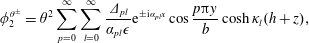 $$\begin{eqnarray}\unicode[STIX]{x1D719}_{2}^{\unicode[STIX]{x1D703}^{\pm }}=\unicode[STIX]{x1D703}^{2}\mathop{\sum }_{p=0}^{\infty }\mathop{\sum }_{l=0}^{\infty }\frac{\unicode[STIX]{x1D6E5}_{pl}}{\unicode[STIX]{x1D6FC}_{pl}\unicode[STIX]{x1D716}}\text{e}^{\pm \text{i}\unicode[STIX]{x1D6FC}_{pl}x}\cos \frac{p\unicode[STIX]{x03C0}y}{b}\cosh \unicode[STIX]{x1D705}_{l}(h+z),\end{eqnarray}$$
while the corresponding free-surface displacement is
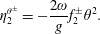 $$\begin{eqnarray}\unicode[STIX]{x1D702}_{2}^{\unicode[STIX]{x1D703}^{\pm }}=-\frac{2\unicode[STIX]{x1D714}}{g}f_{2}^{\pm }\unicode[STIX]{x1D703}^{2}.\end{eqnarray}$$
4.2.2 Response to incident waves –
$\unicode[STIX]{x1D719}^{A^{\pm }}$

This is a simple diffraction problem where the incident wave field forces the gates to move at unison in phase. Decompose
 $\unicode[STIX]{x1D719}^{A^{\pm }}$
as follows:
$\unicode[STIX]{x1D719}^{A^{\pm }}$
as follows:
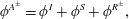 $$\begin{eqnarray}\unicode[STIX]{x1D719}^{A^{\pm }}=\unicode[STIX]{x1D719}^{I}+\unicode[STIX]{x1D719}^{S}+\unicode[STIX]{x1D719}^{R^{\pm }},\end{eqnarray}$$
where
 $$\begin{eqnarray}\unicode[STIX]{x1D719}^{I}=-\frac{\text{i}Ag}{4\unicode[STIX]{x1D714}}\frac{\cosh \unicode[STIX]{x1D705}_{0}(h+z)}{\cosh \unicode[STIX]{x1D705}_{0}h}\text{e}^{-\text{i}\unicode[STIX]{x1D705}_{0}x}\end{eqnarray}$$
is the velocity potential of the incident waves of amplitude
 $A$
,
$A$
,
 $$\begin{eqnarray}\unicode[STIX]{x1D719}^{S}=-\frac{\text{i}Ag}{4\unicode[STIX]{x1D714}}\frac{\cosh \unicode[STIX]{x1D705}_{0}(h+z)}{\cosh \unicode[STIX]{x1D705}_{0}h}\text{e}^{\text{i}\unicode[STIX]{x1D705}_{0}x}\end{eqnarray}$$
is the scattered wave potential, while
 $$\begin{eqnarray}\unicode[STIX]{x1D719}^{R^{\pm }}=\pm \mathop{\sum }_{l=0}^{\infty }\frac{2\unicode[STIX]{x1D714}\unicode[STIX]{x1D703}^{A}D_{l}}{\unicode[STIX]{x1D705}_{l}C_{l}}\cosh \unicode[STIX]{x1D705}_{0}(h+z)\text{e}^{\pm \text{i}\unicode[STIX]{x1D705}_{0}x}\end{eqnarray}$$
is the radiation potential. The angular response
 $\unicode[STIX]{x1D703}^{A}$
is given by
$\unicode[STIX]{x1D703}^{A}$
is given by
 $$\begin{eqnarray}\unicode[STIX]{x1D703}^{A}=\frac{\unicode[STIX]{x1D70C}aAgD_{0}/\cosh \unicode[STIX]{x1D705}_{0}h}{-4\unicode[STIX]{x1D714}^{2}I+C-8\text{i}\unicode[STIX]{x1D714}^{2}\unicode[STIX]{x1D70C}a\displaystyle \mathop{\sum }_{l=0}^{\infty }\frac{D_{l}^{2}}{\unicode[STIX]{x1D705}_{l}C_{l}}}.\end{eqnarray}$$
4.3 The third-order problem
$O(\unicode[STIX]{x1D716}^{2})$

At the order
 $O(\unicode[STIX]{x1D716}^{2})$
, the boundary conditions on the free surface and on the gate array surface are inhomogeneous. Since
$O(\unicode[STIX]{x1D716}^{2})$
, the boundary conditions on the free surface and on the gate array surface are inhomogeneous. Since
 $\unicode[STIX]{x1D714}$
and
$\unicode[STIX]{x1D714}$
and
 $\unicode[STIX]{x1D719}_{1}$
solve the homogeneous problem at the leading order we invoke the solvability condition applying Green’s theorem to
$\unicode[STIX]{x1D719}_{1}$
solve the homogeneous problem at the leading order we invoke the solvability condition applying Green’s theorem to
 $\unicode[STIX]{x1D719}_{1}$
and
$\unicode[STIX]{x1D719}_{1}$
and
 $\unicode[STIX]{x1D719}_{3}$
over the entire fluid domain
$\unicode[STIX]{x1D719}_{3}$
over the entire fluid domain
 $\unicode[STIX]{x1D6FA}^{\pm }$
:
$\unicode[STIX]{x1D6FA}^{\pm }$
:
 $$\begin{eqnarray}\iiint _{\unicode[STIX]{x1D6FA}^{\pm }}(\unicode[STIX]{x1D719}_{1}^{\pm }\unicode[STIX]{x1D6FB}^{2}\unicode[STIX]{x1D719}_{3}^{\pm }-\unicode[STIX]{x1D719}_{3}^{\pm }\unicode[STIX]{x1D6FB}^{2}\unicode[STIX]{x1D719}_{1}^{\pm })\,\text{d}\unicode[STIX]{x1D6FA}^{\pm }=\iint _{\unicode[STIX]{x2202}\unicode[STIX]{x1D6FA}^{\pm }}\left(\unicode[STIX]{x1D719}_{1}\frac{\unicode[STIX]{x2202}\unicode[STIX]{x1D719}_{3}}{\unicode[STIX]{x2202}n}-\unicode[STIX]{x1D719}_{3}\frac{\unicode[STIX]{x2202}\unicode[STIX]{x1D719}_{1}}{\unicode[STIX]{x2202}n}\right)\,\text{d}S^{\pm },\end{eqnarray}$$
where the normal
 $n$
points outward the volume boundaries
$n$
points outward the volume boundaries
 $\unicode[STIX]{x2202}\unicode[STIX]{x1D6FA}$
and the volume integral on the left-hand side is null. Performing straightforward algebra we obtain
$\unicode[STIX]{x2202}\unicode[STIX]{x1D6FA}$
and the volume integral on the left-hand side is null. Performing straightforward algebra we obtain
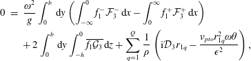 $$\begin{eqnarray}\displaystyle 0 & = & \displaystyle \frac{\unicode[STIX]{x1D714}^{2}}{g}\int _{0}^{b}\,\text{d}y\left(\int _{-\infty }^{0}f_{1}^{-}{\mathcal{F}}_{3}^{-}\,\text{d}x-\int _{0}^{\infty }f_{1}^{+}{\mathcal{F}}_{3}^{+}\,\text{d}x\right)\nonumber\\ \displaystyle & & \displaystyle +\,2\int _{0}^{b}\,\text{d}y\int _{-h}^{0}\overline{f_{1}{\mathcal{G}}_{3}}\,\text{d}z+\mathop{\sum }_{q=1}^{Q}\frac{1}{\unicode[STIX]{x1D70C}}\left(\text{i}{\mathcal{D}}_{3}r_{1q}-\frac{\unicode[STIX]{x1D708}_{pto}r_{1q}^{2}\unicode[STIX]{x1D714}\unicode[STIX]{x1D703}}{\unicode[STIX]{x1D716}^{2}}\right),\end{eqnarray}$$
where the forcing terms
 ${\mathcal{F}}_{3}$
,
${\mathcal{F}}_{3}$
,
 ${\mathcal{G}}_{3}$
,
${\mathcal{G}}_{3}$
,
 ${\mathcal{D}}_{3}$
are given by
${\mathcal{D}}_{3}$
are given by
 $$\begin{eqnarray}{\mathcal{F}}_{3}^{\pm }=\pm \frac{2f_{1}^{\pm }\unicode[STIX]{x1D703}_{t}}{\unicode[STIX]{x1D714}},\end{eqnarray}$$
 $$\begin{eqnarray}\displaystyle {\mathcal{G}}_{3}^{\pm } & = & \displaystyle [\!-r_{1q}\unicode[STIX]{x1D703}^{\ast }(\text{i}\unicode[STIX]{x1D703}^{2}f_{2_{z}}^{\pm }+A\unicode[STIX]{x1D719}_{z}^{A^{\pm }})\mp \text{i}\unicode[STIX]{x1D703}^{A}f_{1_{z}}^{\pm }\unicode[STIX]{x1D703}^{\ast }-r_{1q}\unicode[STIX]{x1D703}_{t}(z+h_{p})\nonumber\\ \displaystyle & & \displaystyle \pm \,d(\unicode[STIX]{x1D703}_{1}^{\ast }\unicode[STIX]{x1D703}_{2})_{t}\! ]H(z+h-c),\end{eqnarray}$$
 $$\begin{eqnarray}\displaystyle {\mathcal{D}}_{3}^{\pm } & = & \displaystyle -\unicode[STIX]{x1D70C}\int _{(q-1)a}^{qa}\,\text{d}y\left\{\int _{-h_{p}}^{0}f_{1}(-6r_{1q}^{2}\unicode[STIX]{x1D703}^{\ast }\unicode[STIX]{x1D703}^{2}\unicode[STIX]{x1D714}-2\text{i}\unicode[STIX]{x1D703}_{t})(z+h_{p})\,\text{d}z\right.\nonumber\\ \displaystyle & & \displaystyle +\left.\,\frac{\unicode[STIX]{x1D714}^{2}f_{1}}{g}\unicode[STIX]{x1D703}^{\ast }\left[-\frac{\unicode[STIX]{x1D714}f_{1}^{2}}{g}\unicode[STIX]{x1D703}^{2}+4h_{p}f_{2}\unicode[STIX]{x1D703}^{2}-4\text{i}h_{p}\unicode[STIX]{x1D719}^{D}\right]\right\}+2\unicode[STIX]{x1D714}Ir_{1q}\text{i}\unicode[STIX]{x1D703}_{t}-\frac{1}{2}gSr_{1q}^{3}\unicode[STIX]{x1D703}^{2}\unicode[STIX]{x1D703}^{\ast }\nonumber\\ \displaystyle & & \displaystyle -\,\unicode[STIX]{x1D70C}\unicode[STIX]{x1D714}\,d\unicode[STIX]{x1D703}^{\ast }\int _{(q-1)a}^{qa}r_{1q}\,\text{d}y\left\{\int _{-h_{p}}^{0}(-4f_{2}\unicode[STIX]{x1D703}^{2}+2\text{i}\unicode[STIX]{x1D719}^{D})\,\text{d}z-3\unicode[STIX]{x1D714}\frac{f_{1}^{2}}{g}\unicode[STIX]{x1D703}^{2}\right\},\end{eqnarray}$$
where
 $\unicode[STIX]{x1D719}^{D}=\unicode[STIX]{x1D719}^{I}+\unicode[STIX]{x1D719}^{S}$
is the diffraction potential and
$\unicode[STIX]{x1D719}^{D}=\unicode[STIX]{x1D719}^{I}+\unicode[STIX]{x1D719}^{S}$
is the diffraction potential and
 $\unicode[STIX]{x1D703}^{\ast }$
denotes the complex conjugate of
$\unicode[STIX]{x1D703}^{\ast }$
denotes the complex conjugate of
 $\unicode[STIX]{x1D703}$
. Solution of the integrals in (4.45) gives the evolution equation of the Stuart–Landau type:
$\unicode[STIX]{x1D703}$
. Solution of the integrals in (4.45) gives the evolution equation of the Stuart–Landau type:
 $$\begin{eqnarray}-\text{i}\unicode[STIX]{x1D703}_{t}=\unicode[STIX]{x1D703}^{2}\unicode[STIX]{x1D703}^{\ast }(c_{N}+\text{i}c_{R})+A\unicode[STIX]{x1D703}^{\ast }c_{F}+\text{i}\unicode[STIX]{x1D703}\unicode[STIX]{x1D708}_{pto}c_{L}.\end{eqnarray}$$
If there is a small detuning
 $2\unicode[STIX]{x0394}\unicode[STIX]{x1D714}$
such that
$2\unicode[STIX]{x0394}\unicode[STIX]{x1D714}$
such that
 $\unicode[STIX]{x0394}\unicode[STIX]{x1D714}/\unicode[STIX]{x1D714}\sim O(\unicode[STIX]{x1D716}^{2})$
, the above equation modifies as follows:
$\unicode[STIX]{x0394}\unicode[STIX]{x1D714}/\unicode[STIX]{x1D714}\sim O(\unicode[STIX]{x1D716}^{2})$
, the above equation modifies as follows:
 $$\begin{eqnarray}-\text{i}\unicode[STIX]{x1D703}_{t}=\unicode[STIX]{x1D703}^{2}\unicode[STIX]{x1D703}^{\ast }(c_{N}+\text{i}c_{R})+A\text{e}^{-2\text{i}\unicode[STIX]{x0394}\unicode[STIX]{x1D714}t}\unicode[STIX]{x1D703}^{\ast }c_{F}+\text{i}\unicode[STIX]{x1D703}\unicode[STIX]{x1D708}_{pto}c_{L}.\end{eqnarray}$$
Through the transformation
 $$\begin{eqnarray}\unicode[STIX]{x1D703}=\overline{\unicode[STIX]{x1D703}}\text{e}^{-\text{i}\unicode[STIX]{x0394}\unicode[STIX]{x1D714}t},\end{eqnarray}$$
equation (4.50) becomes
 $$\begin{eqnarray}-\text{i}\overline{\unicode[STIX]{x1D703}}_{t}=\unicode[STIX]{x0394}\unicode[STIX]{x1D714}\overline{\unicode[STIX]{x1D703}}+\overline{\unicode[STIX]{x1D703}}^{2}\overline{\unicode[STIX]{x1D703}}^{\ast }(c_{N}+\text{i}c_{R})+A\overline{\unicode[STIX]{x1D703}}^{\ast }c_{F}+\text{i}\overline{\unicode[STIX]{x1D703}}\unicode[STIX]{x1D708}_{pto}c_{L}.\end{eqnarray}$$
The coefficient
 $c_{N}$
represents the shift of the trapped mode eigenfrequency from the incident wave frequency,
$c_{N}$
represents the shift of the trapped mode eigenfrequency from the incident wave frequency,
 $c_{R}$
is the radiation damping due to wave radiation at
$c_{R}$
is the radiation damping due to wave radiation at
 $O(\unicode[STIX]{x1D716})$
,
$O(\unicode[STIX]{x1D716})$
,
 $c_{F}$
represents the energy influx by the incident waves while
$c_{F}$
represents the energy influx by the incident waves while
 $c_{L}$
represents damping due to the PTO mechanism.
$c_{L}$
represents damping due to the PTO mechanism.
The coefficients of the evolution equation (4.52)
 $c_{L}$
,
$c_{L}$
,
 $c_{F}$
,
$c_{F}$
,
 $c_{N}+\text{i}c_{R}$
, are given respectively by
$c_{N}+\text{i}c_{R}$
, are given respectively by
 $$\begin{eqnarray}\displaystyle & \displaystyle c_{L}=\frac{\unicode[STIX]{x1D714}}{c_{T}\unicode[STIX]{x1D70C}}\mathop{\sum }_{q=1}^{Q}r_{1q}^{2}, & \displaystyle\end{eqnarray}$$
 $$\begin{eqnarray}\displaystyle & \displaystyle c_{F}=\frac{1}{\text{i}c_{T}}\left(\int _{0}^{b}\,\text{d}y\int _{-h_{p}}^{0}(-f_{1}r_{1q}\unicode[STIX]{x1D719}_{z}^{D}+2\unicode[STIX]{x1D714}\,dr_{1q}^{2}\unicode[STIX]{x1D719}^{D})\,\text{d}z-\int _{0}^{b}2r_{1q}\unicode[STIX]{x1D714}^{2}h_{p}\unicode[STIX]{x1D719}^{D}\frac{f_{1}}{g}\,\text{d}y\right),\qquad & \displaystyle\end{eqnarray}$$
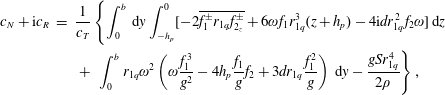 $$\begin{eqnarray}\displaystyle c_{N}+\text{i}c_{R} & = & \displaystyle \frac{1}{c_{T}}\left\{\int _{0}^{b}\,\text{d}y\int _{-h_{p}}^{0}[-2\overline{f_{1}^{\pm }r_{1q}f_{2_{z}}^{\pm }}+6\unicode[STIX]{x1D714}f_{1}r_{1q}^{3}(z+h_{p})-4\text{i}dr_{1q}^{2}f_{2}\unicode[STIX]{x1D714}]\,\text{d}z\right.\nonumber\\ \displaystyle & & \displaystyle \left.+\,\int _{0}^{b}r_{1q}\unicode[STIX]{x1D714}^{2}\left(\unicode[STIX]{x1D714}\frac{f_{1}^{3}}{g^{2}}-4h_{p}\frac{f_{1}}{g}f_{2}+3dr_{1q}\frac{f_{1}^{2}}{g}\right)\,\text{d}y-\frac{gSr_{1q}^{4}}{2\unicode[STIX]{x1D70C}}\right\},\end{eqnarray}$$
with
 $$\begin{eqnarray}c_{T}=\frac{4\unicode[STIX]{x1D714}}{g}\int _{0}^{b}\,\text{d}y\int _{0}^{\infty }f_{1}^{2}\,\text{d}x+2\int _{0}^{b}\,\text{d}y\int _{-h_{p}}^{0}f_{1}r_{1q}(z+h_{p})\,\text{d}z+\mathop{\sum }_{q=1}^{Q}2I\unicode[STIX]{x1D714}r_{1q}^{2}.\end{eqnarray}$$
Computation of
 $c_{F}$
,
$c_{F}$
,
 $c_{N}$
,
$c_{N}$
,
 $c_{R}$
and
$c_{R}$
and
 $c_{T}$
can be evaluated by numerical calculation of the integrals with the known expressions of the integrands.
$c_{T}$
can be evaluated by numerical calculation of the integrals with the known expressions of the integrands.
4.4 Dynamical system analysis for uniform incident waves
By making use of action-angle variables
 $R$
and
$R$
and
 $\unicode[STIX]{x1D713}$
expressed by
$\unicode[STIX]{x1D713}$
expressed by
 $\overline{\unicode[STIX]{x1D703}}=\text{i}\sqrt{R}\text{e}^{\text{i}\unicode[STIX]{x1D713}}$
we obtain the following autonomous dynamical system in
$\overline{\unicode[STIX]{x1D703}}=\text{i}\sqrt{R}\text{e}^{\text{i}\unicode[STIX]{x1D713}}$
we obtain the following autonomous dynamical system in
 $R$
and
$R$
and
 $\unicode[STIX]{x1D713}$
:
$\unicode[STIX]{x1D713}$
:
 $$\begin{eqnarray}\left.\begin{array}{@{}c@{}}R_{t}=-2R(-2c_{R}R+c_{F}A\sin 2\unicode[STIX]{x1D713}+c_{L}\unicode[STIX]{x1D708}_{pto})\\ \unicode[STIX]{x1D713}_{t}=\unicode[STIX]{x0394}\unicode[STIX]{x1D714}+c_{N}R-c_{F}A\cos 2\unicode[STIX]{x1D713}.\end{array}\right\}\end{eqnarray}$$
With the requirement
 $R_{t}=0$
,
$R_{t}=0$
,
 $\unicode[STIX]{x1D713}_{t}=0$
we find at least three fixed points. The trivial fixed point is located at
$\unicode[STIX]{x1D713}_{t}=0$
we find at least three fixed points. The trivial fixed point is located at
 $$\begin{eqnarray}R=0,\quad \unicode[STIX]{x1D713}=(1/2)\cos ^{-1}\frac{\unicode[STIX]{x0394}\unicode[STIX]{x1D714}}{c_{F}A}=\unicode[STIX]{x1D713}^{\ast }.\end{eqnarray}$$
It is easily shown that this point is an unstable saddle for
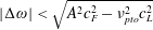 $|\unicode[STIX]{x0394}\unicode[STIX]{x1D714}|<\sqrt{A^{2}c_{F}^{2}-\unicode[STIX]{x1D708}_{pto}^{2}c_{L}^{2}}$
, and a stable fixed point otherwise. The latter condition fixes the threshold of resonance,
$|\unicode[STIX]{x0394}\unicode[STIX]{x1D714}|<\sqrt{A^{2}c_{F}^{2}-\unicode[STIX]{x1D708}_{pto}^{2}c_{L}^{2}}$
, and a stable fixed point otherwise. The latter condition fixes the threshold of resonance,
 $$\begin{eqnarray}A>\frac{c_{L}}{c_{F}}\unicode[STIX]{x1D708}_{pto},\end{eqnarray}$$
i.e. for large values of the PTO coefficient
 $\unicode[STIX]{x1D708}_{pto}$
there is no subharmonic resonance from the rest position and only in-phase motion occurs. Now we seek the non-trivial fixed points which correspond to the roots of the quadratic equation:
$\unicode[STIX]{x1D708}_{pto}$
there is no subharmonic resonance from the rest position and only in-phase motion occurs. Now we seek the non-trivial fixed points which correspond to the roots of the quadratic equation:
 $$\begin{eqnarray}R^{2}(c_{N}^{2}+c_{R}^{2})+2R(c_{R}\unicode[STIX]{x1D708}_{pto}c_{L}+\unicode[STIX]{x0394}\unicode[STIX]{x1D714}c_{N})+\unicode[STIX]{x1D708}_{pto}^{2}c_{L}^{2}+\unicode[STIX]{x0394}\unicode[STIX]{x1D714}^{2}-A^{2}c_{F}^{2}=0,\end{eqnarray}$$
i.e.
 $$\begin{eqnarray}R^{\pm }=\frac{-\unicode[STIX]{x1D708}_{pto}c_{L}c_{R}-c_{N}\unicode[STIX]{x0394}\unicode[STIX]{x1D714}\pm \sqrt{Ac_{F}^{2}(c_{N}^{2}+c_{R}^{2})-\unicode[STIX]{x1D708}_{pto}c_{L}c_{N}+c_{R}\unicode[STIX]{x0394}\unicode[STIX]{x1D714}}}{c_{N}^{2}+c_{R}^{2}}.\end{eqnarray}$$
The latter corresponds to two branches of an ellipse in the plane
 $\unicode[STIX]{x0394}\unicode[STIX]{x1D714},R$
. Since the square root of (4.61) must be real and
$\unicode[STIX]{x0394}\unicode[STIX]{x1D714},R$
. Since the square root of (4.61) must be real and
 $R^{\pm }>0$
, we obtain a single non-trivial fixed point
$R^{\pm }>0$
, we obtain a single non-trivial fixed point
 $R^{+}$
for
$R^{+}$
for
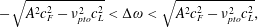 $$\begin{eqnarray}-\sqrt{A^{2}c_{F}^{2}-\unicode[STIX]{x1D708}_{pto}^{2}c_{L}^{2}}<\unicode[STIX]{x0394}\unicode[STIX]{x1D714}<\sqrt{A^{2}c_{F}^{2}-\unicode[STIX]{x1D708}_{pto}^{2}c_{L}^{2}},\end{eqnarray}$$
and the coexistence of two non-trivial fixed points
 $R^{\pm }$
for
$R^{\pm }$
for
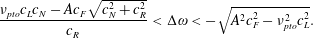 $$\begin{eqnarray}\frac{\unicode[STIX]{x1D708}_{pto}c_{L}c_{N}-Ac_{F}\sqrt{c_{N}^{2}+c_{R}^{2}}}{c_{R}}<\unicode[STIX]{x0394}\unicode[STIX]{x1D714}<-\sqrt{A^{2}c_{F}^{2}-\unicode[STIX]{x1D708}_{pto}^{2}c_{L}^{2}}.\end{eqnarray}$$
The latter holds if
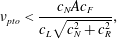 $$\begin{eqnarray}\unicode[STIX]{x1D708}_{pto}<\frac{c_{N}Ac_{F}}{c_{L}\sqrt{c_{N}^{2}+c_{R}^{2}}},\end{eqnarray}$$
this is because
 $\unicode[STIX]{x1D708}_{pto}$
alters the threshold of instability and determines the vanishing of
$\unicode[STIX]{x1D708}_{pto}$
alters the threshold of instability and determines the vanishing of
 $R^{-}$
. Analysis of the Jacobian matrix at the fixed points reveals that
$R^{-}$
. Analysis of the Jacobian matrix at the fixed points reveals that
 $R^{+}$
is stable while
$R^{+}$
is stable while
 $R^{-}$
correspond to an unstable saddle. It is worth evaluating the maximum value of the equilibrium amplitude which corresponds to the maximum of the stable state
$R^{-}$
correspond to an unstable saddle. It is worth evaluating the maximum value of the equilibrium amplitude which corresponds to the maximum of the stable state
 $R^{+}$
. Taking the derivative of
$R^{+}$
. Taking the derivative of
 $R^{+}$
with respect to
$R^{+}$
with respect to
 $\unicode[STIX]{x0394}\unicode[STIX]{x1D714}$
we obtain
$\unicode[STIX]{x0394}\unicode[STIX]{x1D714}$
we obtain
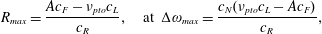 $$\begin{eqnarray}R_{max}=\frac{Ac_{F}-\unicode[STIX]{x1D708}_{pto}c_{L}}{c_{R}},\quad \text{at }\unicode[STIX]{x0394}\unicode[STIX]{x1D714}_{max}=\frac{c_{N}(\unicode[STIX]{x1D708}_{pto}c_{L}-Ac_{F})}{c_{R}},\end{eqnarray}$$
or in terms of the modal amplitude:
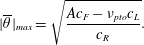 $$\begin{eqnarray}|\overline{\unicode[STIX]{x1D703}}|_{max}=\sqrt{\frac{Ac_{F}-\unicode[STIX]{x1D708}_{pto}c_{L}}{c_{R}}}.\end{eqnarray}$$
Once
 $|\overline{\unicode[STIX]{x1D703}}|$
is evaluated, the average generated power by the array due to subharmonic resonance of the natural mode is given by
$|\overline{\unicode[STIX]{x1D703}}|$
is evaluated, the average generated power by the array due to subharmonic resonance of the natural mode is given by
 $$\begin{eqnarray}P_{s}(\unicode[STIX]{x1D708}_{pto},R^{+})=\frac{\unicode[STIX]{x1D714}}{2\unicode[STIX]{x03C0}}\int _{0}^{2\unicode[STIX]{x03C0}/\unicode[STIX]{x1D714}}\unicode[STIX]{x1D708}_{pto}\mathop{\sum }_{q=1}^{Q}\left(\frac{\text{d}\unicode[STIX]{x1D6E9}_{q}}{\text{d}t}\right)^{2}\,\text{d}t=2\unicode[STIX]{x1D708}_{pto}(\unicode[STIX]{x1D714}+\unicode[STIX]{x0394}\unicode[STIX]{x1D714})^{2}\mathop{\sum }_{q=1}^{Q}r_{1q}^{2}R^{+}.\end{eqnarray}$$
The maximum of
 $P_{s}$
depends on
$P_{s}$
depends on
 $\unicode[STIX]{x0394}\unicode[STIX]{x1D714}$
and
$\unicode[STIX]{x0394}\unicode[STIX]{x1D714}$
and
 $\unicode[STIX]{x1D708}_{pto}$
and cannot be found analytically. Numerical calculation of (4.67) reveals that a good approximation consists in finding the optimal value of
$\unicode[STIX]{x1D708}_{pto}$
and cannot be found analytically. Numerical calculation of (4.67) reveals that a good approximation consists in finding the optimal value of
 $\unicode[STIX]{x1D708}_{pto}$
which maximizes the generated power at
$\unicode[STIX]{x1D708}_{pto}$
which maximizes the generated power at
 $\unicode[STIX]{x0394}\unicode[STIX]{x1D714}=\unicode[STIX]{x0394}\unicode[STIX]{x1D714}_{max}$
where the gate oscillation is maximum. So we impose the derivative of (4.67) with respect to
$\unicode[STIX]{x0394}\unicode[STIX]{x1D714}=\unicode[STIX]{x0394}\unicode[STIX]{x1D714}_{max}$
where the gate oscillation is maximum. So we impose the derivative of (4.67) with respect to
 $\unicode[STIX]{x1D708}_{pto}$
evaluated at
$\unicode[STIX]{x1D708}_{pto}$
evaluated at
 $\unicode[STIX]{x0394}\unicode[STIX]{x1D714}_{max}$
to be zero:
$\unicode[STIX]{x0394}\unicode[STIX]{x1D714}_{max}$
to be zero:
 $$\begin{eqnarray}\left.\frac{\text{d}P_{s}}{\text{d}\unicode[STIX]{x1D708}_{pto}}\right|_{\unicode[STIX]{x0394}\unicode[STIX]{x1D714}=\unicode[STIX]{x0394}\unicode[STIX]{x1D714}_{max}}=0.\end{eqnarray}$$
Solution of the latter equation yields a criterion to find the optimal value of the PTO coefficient which maximizes the power output:
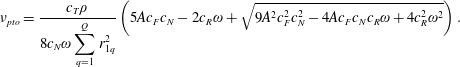 $$\begin{eqnarray}\unicode[STIX]{x1D708}_{pto}=\frac{c_{T}\unicode[STIX]{x1D70C}}{8c_{N}\unicode[STIX]{x1D714}\displaystyle \mathop{\sum }_{q=1}^{Q}r_{1q}^{2}}\left(5Ac_{F}c_{N}-2c_{R}\unicode[STIX]{x1D714}+\sqrt{9A^{2}c_{F}^{2}c_{N}^{2}-4Ac_{F}c_{N}c_{R}\unicode[STIX]{x1D714}+4c_{R}^{2}\unicode[STIX]{x1D714}^{2}}\right).\end{eqnarray}$$
Finally we assess the maximum efficiency of the system by considering the capture width ratio
 ${\mathcal{C}}^{F}$
(Mei et al.
Reference Mei, Stiassnie and Yue2005) defined as the ratio between
${\mathcal{C}}^{F}$
(Mei et al.
Reference Mei, Stiassnie and Yue2005) defined as the ratio between
 $P_{s}$
and the incident wave energy flux per array width
$P_{s}$
and the incident wave energy flux per array width
 $b$
(Michele et al.
Reference Michele, Sammarco and d’Errico2016b
):
$b$
(Michele et al.
Reference Michele, Sammarco and d’Errico2016b
):
 $$\begin{eqnarray}{\mathcal{C}}^{F}=\frac{P_{s}}{EC_{g}b},\end{eqnarray}$$
where
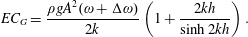 $$\begin{eqnarray}EC_{G}=\frac{\unicode[STIX]{x1D70C}gA^{2}(\unicode[STIX]{x1D714}+\unicode[STIX]{x0394}\unicode[STIX]{x1D714})}{2k}\left(1+\frac{2kh}{\sinh 2kh}\right).\end{eqnarray}$$
In the latter,
 $C_{G}$
is the group velocity and
$C_{G}$
is the group velocity and
 $k$
the wavenumber related to the frequency
$k$
the wavenumber related to the frequency
 $2(\unicode[STIX]{x1D714}+\unicode[STIX]{x0394}\unicode[STIX]{x1D714})$
.
$2(\unicode[STIX]{x1D714}+\unicode[STIX]{x0394}\unicode[STIX]{x1D714})$
.
4.5 The non-autonomous dynamical system for modulated incident waves
In this section we investigate the effects of a modulation of the incident wave envelope on the dynamics and power generated by the array. Let us assume
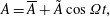 $$\begin{eqnarray}A=\overline{A}+\tilde{A}\cos \unicode[STIX]{x1D6FA}t,\end{eqnarray}$$
where
 $\overline{A}$
is the constant amplitude of the short waves, while
$\overline{A}$
is the constant amplitude of the short waves, while
 $\tilde{A}$
and
$\tilde{A}$
and
 $\unicode[STIX]{x1D6FA}$
are respectively the amplitude and frequency of the modulation with order
$\unicode[STIX]{x1D6FA}$
are respectively the amplitude and frequency of the modulation with order
 $O(\unicode[STIX]{x1D716}^{2})$
. The evolution equation now includes a forcing term in time and becomes
$O(\unicode[STIX]{x1D716}^{2})$
. The evolution equation now includes a forcing term in time and becomes
 $$\begin{eqnarray}-\text{i}\overline{\unicode[STIX]{x1D703}}_{t}=\unicode[STIX]{x0394}\unicode[STIX]{x1D714}\overline{\unicode[STIX]{x1D703}}+\overline{\unicode[STIX]{x1D703}}^{2}\overline{\unicode[STIX]{x1D703}}^{\ast }(c_{N}+\text{i}c_{R})+(\overline{A}+\tilde{A}\cos \unicode[STIX]{x1D6FA}t)\overline{\unicode[STIX]{x1D703}}^{\ast }c_{F}+\text{i}\overline{\unicode[STIX]{x1D703}}c_{L}.\end{eqnarray}$$
In action-angle coordinates the latter equation reads
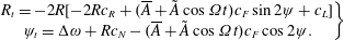 $$\begin{eqnarray}\left.\begin{array}{@{}c@{}}R_{t}=-2R[-2Rc_{R}+(\overline{A}+\tilde{A}\cos \unicode[STIX]{x1D6FA}t)c_{F}\sin 2\unicode[STIX]{x1D713}+c_{L}]\\ \unicode[STIX]{x1D713}_{t}=\unicode[STIX]{x0394}\unicode[STIX]{x1D714}+Rc_{N}-(\overline{A}+\tilde{A}\cos \unicode[STIX]{x1D6FA}t)c_{F}\cos 2\unicode[STIX]{x1D713}.\end{array}\right\}\end{eqnarray}$$
The latter non-autonomous system is similar to that for Venice gates (Sammarco et al.
Reference Sammarco, Tran, Gottlieb and Mei1997b
) and can exhibit chaos for a certain range of the long wave amplitude
 $\tilde{A}$
. There are different theoretical criteria to determine under what conditions the response of a dynamical system becomes chaotic. In this paper we make use of the Melnikov method. This mathematical technique allows us to predict global chaos and is based on the search of horseshoe maps and homoclinic/heteroclinic orbits of the associated undamped Hamiltonian system (Guckenheimer & Holmes Reference Guckenheimer and Holmes1983). Let us assume the following variables:
$\tilde{A}$
. There are different theoretical criteria to determine under what conditions the response of a dynamical system becomes chaotic. In this paper we make use of the Melnikov method. This mathematical technique allows us to predict global chaos and is based on the search of horseshoe maps and homoclinic/heteroclinic orbits of the associated undamped Hamiltonian system (Guckenheimer & Holmes Reference Guckenheimer and Holmes1983). Let us assume the following variables:
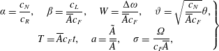 $$\begin{eqnarray}\left.\begin{array}{@{}c@{}}\displaystyle \unicode[STIX]{x1D6FC}=\frac{c_{N}}{c_{R}},\quad \unicode[STIX]{x1D6FD}=\frac{c_{L}}{\overline{A}c_{F}},\quad W=\frac{\unicode[STIX]{x0394}\unicode[STIX]{x1D714}}{\overline{A}c_{F}},\quad \unicode[STIX]{x1D717}=\sqrt{\frac{c_{N}}{\overline{A}c_{F}}}\unicode[STIX]{x1D703},\\ \displaystyle T=\overline{A}c_{F}t,\quad a=\frac{\tilde{A}}{\overline{A}},\quad \unicode[STIX]{x1D70E}=\frac{\unicode[STIX]{x1D6FA}}{c_{F}\overline{A}},\end{array}\right\}\end{eqnarray}$$
and the damping and forcing terms to be
 $O(\unicode[STIX]{x1D6FF})$
with
$O(\unicode[STIX]{x1D6FF})$
with
 $\unicode[STIX]{x1D6FF}\ll 1$
. By denoting with
$\unicode[STIX]{x1D6FF}\ll 1$
. By denoting with
 $\unicode[STIX]{x1D717}=\text{i}\sqrt{R^{\prime }}\text{e}^{\text{i}\unicode[STIX]{x1D713}^{\prime }}$
, the system (4.74) can be rewritten in the form
$\unicode[STIX]{x1D717}=\text{i}\sqrt{R^{\prime }}\text{e}^{\text{i}\unicode[STIX]{x1D713}^{\prime }}$
, the system (4.74) can be rewritten in the form
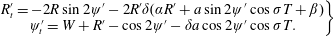 $$\begin{eqnarray}\left.\begin{array}{@{}c@{}}R_{t}^{\prime }=-2R\sin 2\unicode[STIX]{x1D713}^{\prime }-2R^{\prime }\unicode[STIX]{x1D6FF}(\unicode[STIX]{x1D6FC}R^{\prime }+a\sin 2\unicode[STIX]{x1D713}^{\prime }\cos \unicode[STIX]{x1D70E}T+\unicode[STIX]{x1D6FD})\\ \unicode[STIX]{x1D713}_{t}^{\prime }=W+R^{\prime }-\cos 2\unicode[STIX]{x1D713}^{\prime }-\unicode[STIX]{x1D6FF}a\cos 2\unicode[STIX]{x1D713}^{\prime }\cos \unicode[STIX]{x1D70E}T.\end{array}\right\}\end{eqnarray}$$
The Hamiltonian function of the unforced system is then given by
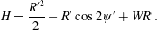 $$\begin{eqnarray}H=\frac{R^{\prime 2}}{2}-R^{\prime }\cos 2\unicode[STIX]{x1D713}^{\prime }+WR^{\prime }.\end{eqnarray}$$
At
 $O(1)$
the system (4.76) admits three fixed points:
$O(1)$
the system (4.76) admits three fixed points:
 $$\begin{eqnarray}O=\{0,{\textstyle \frac{1}{2}}\cos ^{-1}W\},\quad s=\{1-W,0\},\quad u=\{-1-W,0\},\end{eqnarray}$$
where
 $O$
is an unstable saddle for
$O$
is an unstable saddle for
 $|W|<1$
and a centre if
$|W|<1$
and a centre if
 $|W|>1$
, the fixed point
$|W|>1$
, the fixed point
 $s$
is a centre and exist for
$s$
is a centre and exist for
 $W<1$
while
$W<1$
while
 $u$
is an unstable saddle and exist for
$u$
is an unstable saddle and exist for
 $W<-1$
. Because heteroclinic tangle is difficult to excite experimentally (Sammarco et al.
Reference Sammarco, Tran, Gottlieb and Mei1997b
), we focus our attention to the bifurcation of homoclinic paths assuming
$W<-1$
. Because heteroclinic tangle is difficult to excite experimentally (Sammarco et al.
Reference Sammarco, Tran, Gottlieb and Mei1997b
), we focus our attention to the bifurcation of homoclinic paths assuming
 $W=0$
. In this case the homoclinic orbit has the equation
$W=0$
. In this case the homoclinic orbit has the equation
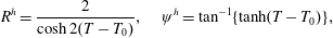 $$\begin{eqnarray}R^{h}=\frac{2}{\cosh 2(T-T_{0})},\quad \unicode[STIX]{x1D713}^{h}=\tan ^{-1}\{\tanh (T-T_{0})\},\end{eqnarray}$$
and the corresponding Melnikov function is given by
 $$\begin{eqnarray}M(T_{0})=\int _{-\infty }^{\infty }2R^{h}[a_{1}R^{h}\sin 2\unicode[STIX]{x1D713}^{h}\cos \unicode[STIX]{x1D70E}T+(R^{h}-\cos 2\unicode[STIX]{x1D713}^{h})(\unicode[STIX]{x1D6FC}_{1}R^{h}+\unicode[STIX]{x1D6FD}_{1})]\,\text{d}T,\end{eqnarray}$$
where
 $$\begin{eqnarray}(\unicode[STIX]{x1D6FC}_{1},\unicode[STIX]{x1D6FD}_{1},a1)=\frac{(\unicode[STIX]{x1D6FC},\unicode[STIX]{x1D6FD},a)}{\unicode[STIX]{x1D707}}.\end{eqnarray}$$
Homoclinic tangle occurs when
 $M(T_{0})$
has a simple zero. The integral (4.80) can be evaluated analytically, and gives the lower threshold in terms of the modulated amplitude
$M(T_{0})$
has a simple zero. The integral (4.80) can be evaluated analytically, and gives the lower threshold in terms of the modulated amplitude
 $\tilde{A}$
to give rise to horseshoe structures in the neighbourhood of the homoclinic orbit
$\tilde{A}$
to give rise to horseshoe structures in the neighbourhood of the homoclinic orbit
 $R^{h},\unicode[STIX]{x1D713}^{h}$
:
$R^{h},\unicode[STIX]{x1D713}^{h}$
:
 $$\begin{eqnarray}\tilde{A}=\frac{4\overline{A}^{3}c_{F}^{2}}{\unicode[STIX]{x03C0}\unicode[STIX]{x1D6FA}^{2}}\left(\frac{\unicode[STIX]{x03C0}c_{R}}{c_{N}}+\frac{2c_{L}}{\overline{A}c_{F}}\right)\sinh \frac{\unicode[STIX]{x03C0}\unicode[STIX]{x1D6FA}}{4\overline{A}c_{F}}.\end{eqnarray}$$
Note that the smaller the damping due to
 $O(\unicode[STIX]{x1D716})$
radiated waves and PTO coefficient, the lower is the threshold. Moreover, taking the limit of (4.82) for
$O(\unicode[STIX]{x1D716})$
radiated waves and PTO coefficient, the lower is the threshold. Moreover, taking the limit of (4.82) for
 $\unicode[STIX]{x1D6FA}\rightarrow (0,\infty )$
we obtain that
$\unicode[STIX]{x1D6FA}\rightarrow (0,\infty )$
we obtain that
 $\tilde{A}$
tends to infinity and chaos is not generated.
$\tilde{A}$
tends to infinity and chaos is not generated.
4.6 Results for uniform incident waves and
$Q=2$

Here we discuss the theoretical results of the previous section for the case of
 $Q=2$
gates with channel and array dimensions listed in table 3. Let us assume the amplitude of the incident wave
$Q=2$
gates with channel and array dimensions listed in table 3. Let us assume the amplitude of the incident wave
 $A=0.1$
m. Solution of the
$A=0.1$
m. Solution of the
 $O(1)$
problem yields a trapped mode with eigenvector
$O(1)$
problem yields a trapped mode with eigenvector
 $r_{1q}=\{1,-1\}$
. The values of the coefficients
$r_{1q}=\{1,-1\}$
. The values of the coefficients
 $c_{L}$
,
$c_{L}$
,
 $c_{N}$
,
$c_{N}$
,
 $c_{R}$
and
$c_{R}$
and
 $c_{F}$
with respect to the eigenfrequency
$c_{F}$
with respect to the eigenfrequency
 $\unicode[STIX]{x1D714}$
are shown in figure 2. All the coefficients show similar behaviour, i.e. they increase with the eigenfrequency of the mode.
$\unicode[STIX]{x1D714}$
are shown in figure 2. All the coefficients show similar behaviour, i.e. they increase with the eigenfrequency of the mode.
Table 3. Flap and channel dimensions.
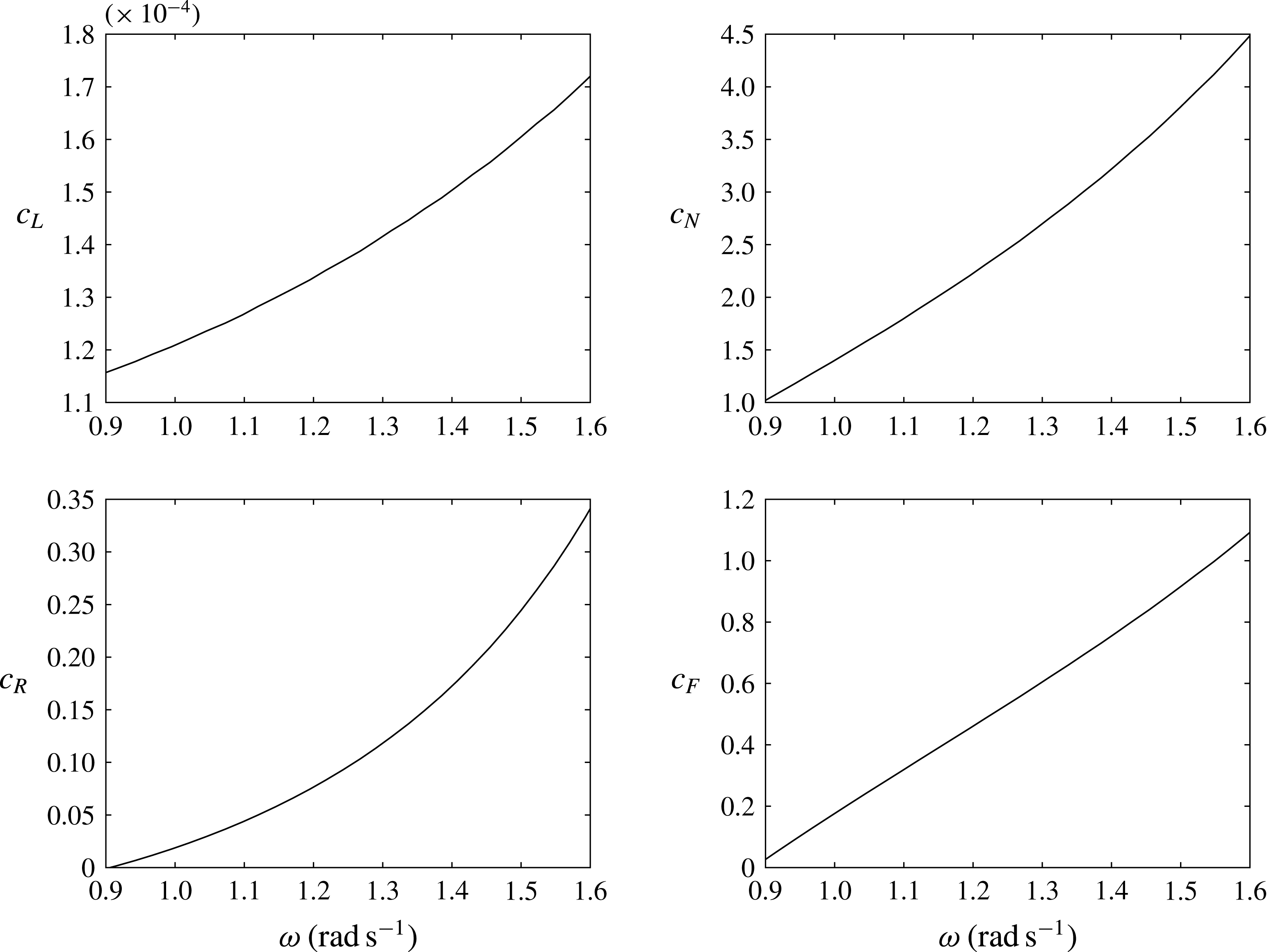
Figure 2. Behaviour of the coefficients of the evolution equation versus the eigenfrequency
 $\unicode[STIX]{x1D714}$
.
$\unicode[STIX]{x1D714}$
.
In figure 3 we show the dependence of the maximum value of the capture factor
 ${\mathcal{C}}_{max}^{F}$
(4.70) and of the optimal value of the PTO coefficient (4.69) on the eigenfrequency
${\mathcal{C}}_{max}^{F}$
(4.70) and of the optimal value of the PTO coefficient (4.69) on the eigenfrequency
 $\unicode[STIX]{x1D714}$
. The larger the eigenfrequency the larger the efficiency of the system, hence gates with large buoyancy (large eigenfrequency
$\unicode[STIX]{x1D714}$
. The larger the eigenfrequency the larger the efficiency of the system, hence gates with large buoyancy (large eigenfrequency
 $\unicode[STIX]{x1D714}$
) are more efficient than heavier gates with large inertia. Moreover, figure 3(a) reveals that the capture factor can be larger than
$\unicode[STIX]{x1D714}$
) are more efficient than heavier gates with large inertia. Moreover, figure 3(a) reveals that the capture factor can be larger than
 $0.5$
. This latter value corresponds to the maximum of a two-dimensional wave absorber working in synchronous resonance conditions with PTO coefficient equal to the radiation damping (Mei et al.
Reference Mei, Stiassnie and Yue2005). Hence, nonlinear resonance has a significant beneficial effect on power extraction.
$0.5$
. This latter value corresponds to the maximum of a two-dimensional wave absorber working in synchronous resonance conditions with PTO coefficient equal to the radiation damping (Mei et al.
Reference Mei, Stiassnie and Yue2005). Hence, nonlinear resonance has a significant beneficial effect on power extraction.

Figure 3. (a) Maximum of the capture factor
 ${\mathcal{C}}_{max}^{F}$
versus the eigenfrequency of the array
${\mathcal{C}}_{max}^{F}$
versus the eigenfrequency of the array
 $\unicode[STIX]{x1D714}$
. The capture factor reaches values larger than 0.5, i.e. the maximum that can be reached with synchronous motion only. (b) The optimal value of
$\unicode[STIX]{x1D714}$
. The capture factor reaches values larger than 0.5, i.e. the maximum that can be reached with synchronous motion only. (b) The optimal value of
 $\unicode[STIX]{x1D708}_{pto}$
versus eigenfrequency
$\unicode[STIX]{x1D708}_{pto}$
versus eigenfrequency
 $\unicode[STIX]{x1D714}$
. The power take-off increases with
$\unicode[STIX]{x1D714}$
. The power take-off increases with
 $\unicode[STIX]{x1D714}$
.
$\unicode[STIX]{x1D714}$
.
We now examine the behaviour of the bandwidth of instability expressed by (4.62) on the eigenfrequency
 $\unicode[STIX]{x1D714}$
for the optimal values of
$\unicode[STIX]{x1D714}$
for the optimal values of
 $\unicode[STIX]{x1D708}_{pto}$
(see figure 4). For large values of the inertia, i.e. small eigenfrequencies
$\unicode[STIX]{x1D708}_{pto}$
(see figure 4). For large values of the inertia, i.e. small eigenfrequencies
 $\unicode[STIX]{x1D714}$
, the frequency band of instability approaches zero. Hence heavier gates are more difficult to resonate. Conversely, gates characterized by large values of the buoyancy can be easily resonated because the bandwidth of instability tends to increase. In summary, from a nonlinear point of view maximization of the performance of an array of OWCSs can be reached by choosing gates with large hydrodynamic stiffness.
$\unicode[STIX]{x1D714}$
, the frequency band of instability approaches zero. Hence heavier gates are more difficult to resonate. Conversely, gates characterized by large values of the buoyancy can be easily resonated because the bandwidth of instability tends to increase. In summary, from a nonlinear point of view maximization of the performance of an array of OWCSs can be reached by choosing gates with large hydrodynamic stiffness.

Figure 4. Bandwidth of instability versus the eigenfrequency of the array
 $\unicode[STIX]{x1D714}$
. Gates with small inertia
$\unicode[STIX]{x1D714}$
. Gates with small inertia
 $I$
and large buoyancy
$I$
and large buoyancy
 $C$
increase the eigenfrequency of the mode and render the subharmonic resonance more observable and efficient to extract power from water waves.
$C$
increase the eigenfrequency of the mode and render the subharmonic resonance more observable and efficient to extract power from water waves.
Let us fix the eigenfrequency
 $\unicode[STIX]{x1D714}=1.5~\text{rad}~\text{s}^{-1}$
. The corresponding values of the coefficients of the evolution equation are (see also figure 2):
$\unicode[STIX]{x1D714}=1.5~\text{rad}~\text{s}^{-1}$
. The corresponding values of the coefficients of the evolution equation are (see also figure 2):
 $$\begin{eqnarray}c_{L}=1.6\times 10^{-4},\quad c_{N}=3.81,\quad c_{R}=0.24,\quad c_{F}=0.91,\end{eqnarray}$$
while the value of
 $\unicode[STIX]{x1D708}_{pto}$
is chosen following (4.69) (see figure 3
b), i.e.
$\unicode[STIX]{x1D708}_{pto}$
is chosen following (4.69) (see figure 3
b), i.e.
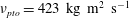 $\unicode[STIX]{x1D708}_{pto}=423~\text{kg}~\text{m}^{2}~\text{s}^{-1}$
. Figure 5 shows the bifurcation diagram describing the dependence of the unstable and stable equilibria
$\unicode[STIX]{x1D708}_{pto}=423~\text{kg}~\text{m}^{2}~\text{s}^{-1}$
. Figure 5 shows the bifurcation diagram describing the dependence of the unstable and stable equilibria
 $R^{\pm }$
on
$R^{\pm }$
on
 $\unicode[STIX]{x0394}\unicode[STIX]{x1D714}$
. The ellipse is inclined to the left hence the system behaves like a Duffing oscillator with soft spring. Similar behaviour has been already obtained for the subharmonic resonance of Venice gates analysed by Sammarco et al. (Reference Sammarco, Tran and Mei1997a
,Reference Sammarco, Tran, Gottlieb and Mei
b
).
$\unicode[STIX]{x0394}\unicode[STIX]{x1D714}$
. The ellipse is inclined to the left hence the system behaves like a Duffing oscillator with soft spring. Similar behaviour has been already obtained for the subharmonic resonance of Venice gates analysed by Sammarco et al. (Reference Sammarco, Tran and Mei1997a
,Reference Sammarco, Tran, Gottlieb and Mei
b
).

Figure 5. Bifurcation diagram of stable/unstable branches for the eigenfrequency of the natural mode
 $\unicode[STIX]{x1D714}=1.5~\text{rad}~\text{s}^{-1}$
: – – –, unstable branch; ——, stable branch.
$\unicode[STIX]{x1D714}=1.5~\text{rad}~\text{s}^{-1}$
: – – –, unstable branch; ——, stable branch.
Figure 6 shows the behaviour of the capture factor
 ${\mathcal{C}}^{F}$
given by (4.70) versus the detuning
${\mathcal{C}}^{F}$
given by (4.70) versus the detuning
 $\unicode[STIX]{x0394}\unicode[STIX]{x1D714}$
. The maximum capture factor that can be reached is
$\unicode[STIX]{x0394}\unicode[STIX]{x1D714}$
. The maximum capture factor that can be reached is
 ${\mathcal{C}}^{F}\sim 1$
(see also figure 3
a for
${\mathcal{C}}^{F}\sim 1$
(see also figure 3
a for
 $\unicode[STIX]{x1D714}\sim 1.5~\text{rad}~\text{s}^{-1}$
), i.e. twice the size of the maximum possible for linear synchronous excitation in a channel (Mei et al.
Reference Mei, Stiassnie and Yue2005).
$\unicode[STIX]{x1D714}\sim 1.5~\text{rad}~\text{s}^{-1}$
), i.e. twice the size of the maximum possible for linear synchronous excitation in a channel (Mei et al.
Reference Mei, Stiassnie and Yue2005).
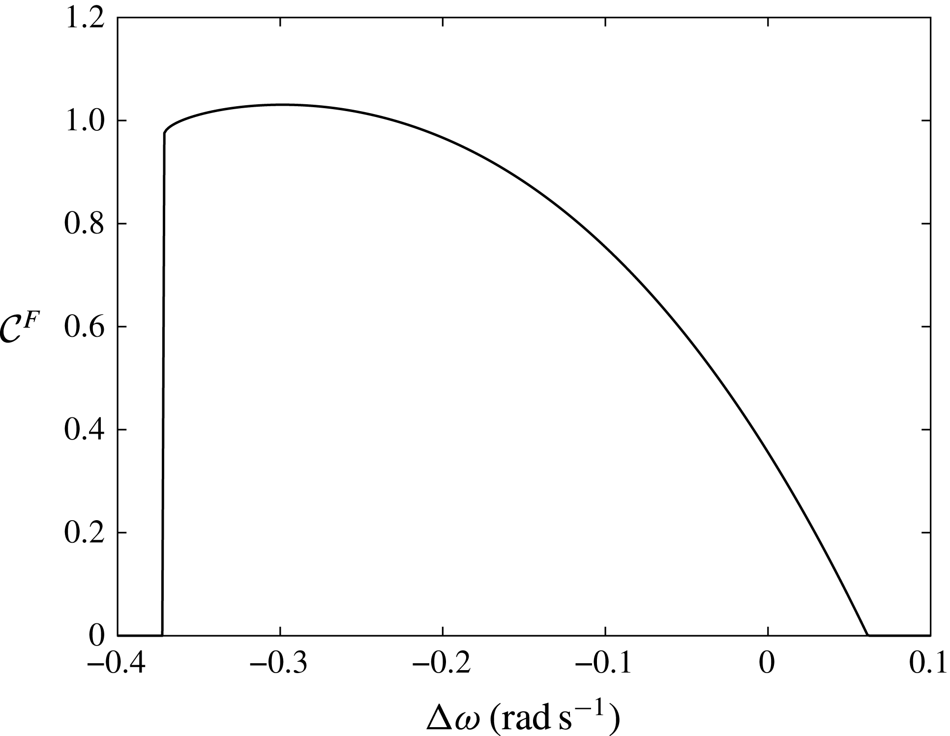
Figure 6. Behaviour of the capture factor
 ${\mathcal{C}}^{F}$
versus detuning
${\mathcal{C}}^{F}$
versus detuning
 $\unicode[STIX]{x0394}\unicode[STIX]{x1D714}$
.
$\unicode[STIX]{x0394}\unicode[STIX]{x1D714}$
.
4.7 Results for modulated incident waves and
$Q=2$

In this section we show the behaviour of the array in modulated incident waves with
 $\overline{A}=0.1$
m. To investigate the effects of the gate stiffness on the minimum of the Melnikov function, consider the geometrical characteristics listed in table 3 and two different values of the eigenfrequency, that is,
$\overline{A}=0.1$
m. To investigate the effects of the gate stiffness on the minimum of the Melnikov function, consider the geometrical characteristics listed in table 3 and two different values of the eigenfrequency, that is,
 $\unicode[STIX]{x1D714}_{1}=1.5$
and
$\unicode[STIX]{x1D714}_{1}=1.5$
and
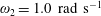 $\unicode[STIX]{x1D714}_{2}=1.0~\text{rad}~\text{s}^{-1}$
. The respective values of the coefficients are
$\unicode[STIX]{x1D714}_{2}=1.0~\text{rad}~\text{s}^{-1}$
. The respective values of the coefficients are
 $$\begin{eqnarray}\left.\begin{array}{@{}c@{}}c_{L1}=1.6\times 10^{-4},\quad c_{N1}=3.81,\quad c_{R1}=0.24,\quad c_{F1}=0.91,\\ c_{L2}=1.2\times 10^{-4},\quad c_{N2}=1.38,\quad c_{R2}=0.02,\quad c_{F2}=0.17.\end{array}\right\}\end{eqnarray}$$
For each system we choose the PTO coefficient that satisfies (4.69) and maximizes power output. We obtain
 $$\begin{eqnarray}\unicode[STIX]{x1D708}_{1}=423,\quad \unicode[STIX]{x1D708}_{2}=111~\text{kg}~\text{m}^{2}~\text{s}^{-1}.\end{eqnarray}$$
Once the coefficients are evaluated, we assume
 $\unicode[STIX]{x0394}\unicode[STIX]{x1D714}=0$
and derive the threshold for global chaos that can lead to homoclinic tangle. Figure 7 shows the dependence of the amplitude
$\unicode[STIX]{x0394}\unicode[STIX]{x1D714}=0$
and derive the threshold for global chaos that can lead to homoclinic tangle. Figure 7 shows the dependence of the amplitude
 $\tilde{A}$
on the long-wave frequency
$\tilde{A}$
on the long-wave frequency
 $\unicode[STIX]{x1D6FA}$
for both systems. The minimum value shifts to the right with increasing eigenfrequency of the array. Note that the bandwidth for gates with small buoyancy is narrower than that for gates characterized by small inertia. These results demonstrate that with respect to the case of heavier gates, systems with larger eigenfrequencies (more buoyant) can exhibit chaos for a broader range of long-wave forcing frequencies.
$\unicode[STIX]{x1D6FA}$
for both systems. The minimum value shifts to the right with increasing eigenfrequency of the array. Note that the bandwidth for gates with small buoyancy is narrower than that for gates characterized by small inertia. These results demonstrate that with respect to the case of heavier gates, systems with larger eigenfrequencies (more buoyant) can exhibit chaos for a broader range of long-wave forcing frequencies.

Figure 7. Melnikov criterion for determining lower bound of chaos in the plane
 $\tilde{A}{-}\unicode[STIX]{x1D6FA}$
. Location of the minima depends on the eigenfrequency
$\tilde{A}{-}\unicode[STIX]{x1D6FA}$
. Location of the minima depends on the eigenfrequency
 $\unicode[STIX]{x1D714}$
and tends to zero with the gate inertia. Moreover note that
$\unicode[STIX]{x1D714}$
and tends to zero with the gate inertia. Moreover note that
 $\tilde{A}\rightarrow \infty$
for
$\tilde{A}\rightarrow \infty$
for
 $\unicode[STIX]{x1D6FA}\rightarrow (0,\infty )$
and chaotic response becomes impracticable.
$\unicode[STIX]{x1D6FA}\rightarrow (0,\infty )$
and chaotic response becomes impracticable.

Figure 8. Gate array response at
 $\tilde{A}=0.05~\text{m}$
. Synchronous response. (a) Phase plane
$\tilde{A}=0.05~\text{m}$
. Synchronous response. (a) Phase plane
 $X{-}Y$
and Poincaré map for the evolution of
$X{-}Y$
and Poincaré map for the evolution of
 $\overline{\unicode[STIX]{x1D703}}$
; (b) power spectrum of the gate oscillation.
$\overline{\unicode[STIX]{x1D703}}$
; (b) power spectrum of the gate oscillation.
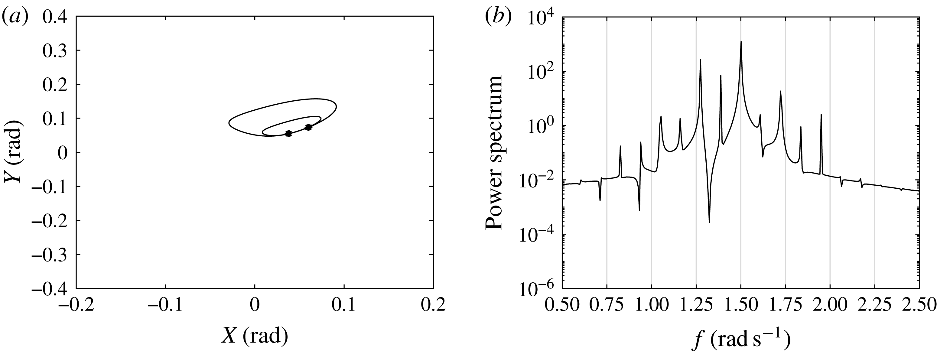
Figure 9. Subharmonic response at
 $\tilde{A}=0.14~\text{m}$
.
$\tilde{A}=0.14~\text{m}$
.
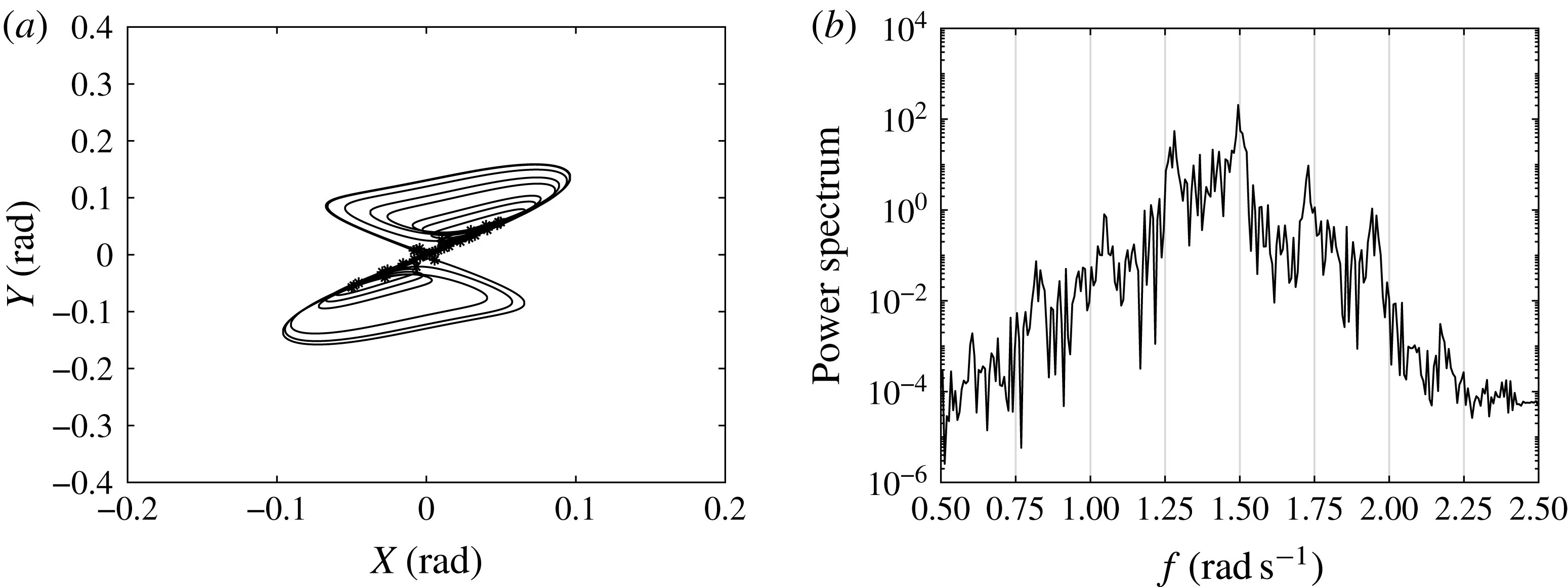
Figure 10. Chaos at
 $\tilde{A}=0.2~\text{m}$
.
$\tilde{A}=0.2~\text{m}$
.
Now integrate system (4.74) numerically and investigate the occurrence of bifurcation scenarios with increasing amplitude
 $\tilde{A}$
. Let us assume the eigenfrequency of the array to be
$\tilde{A}$
. Let us assume the eigenfrequency of the array to be
 $\unicode[STIX]{x1D714}=1.5~\text{rad}~\text{s}^{-1}$
and fix the frequency of the long wave which corresponds to the minimum of the threshold shown in figure 7, i.e.
$\unicode[STIX]{x1D714}=1.5~\text{rad}~\text{s}^{-1}$
and fix the frequency of the long wave which corresponds to the minimum of the threshold shown in figure 7, i.e.
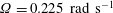 $\unicode[STIX]{x1D6FA}=0.225~\text{rad}~\text{s}^{-1}$
. In order to follow bifurcation patterns we use the Poincaré map sampling time series of the gate envelope response
$\unicode[STIX]{x1D6FA}=0.225~\text{rad}~\text{s}^{-1}$
. In order to follow bifurcation patterns we use the Poincaré map sampling time series of the gate envelope response
 $\overline{\unicode[STIX]{x1D703}}$
at times
$\overline{\unicode[STIX]{x1D703}}$
at times
 $t=2\unicode[STIX]{x03C0}n/\unicode[STIX]{x1D6FA}$
,
$t=2\unicode[STIX]{x03C0}n/\unicode[STIX]{x1D6FA}$
,
 $n=1,2,3\ldots ,$
once transient motion disappears. To better analyse
$n=1,2,3\ldots ,$
once transient motion disappears. To better analyse
 $\overline{\unicode[STIX]{x1D703}}$
we use the definition
$\overline{\unicode[STIX]{x1D703}}$
we use the definition
 $\overline{\unicode[STIX]{x1D703}}=X+\text{i}Y$
separating real and imaginary parts. Moreover, the output of (4.74) includes several harmonics, hence we further investigate the time series of the gate response
$\overline{\unicode[STIX]{x1D703}}=X+\text{i}Y$
separating real and imaginary parts. Moreover, the output of (4.74) includes several harmonics, hence we further investigate the time series of the gate response
 $\unicode[STIX]{x1D6E9}(t)$
looking at its power spectrum (Jordan & Smith Reference Jordan and Smith2011). For
$\unicode[STIX]{x1D6E9}(t)$
looking at its power spectrum (Jordan & Smith Reference Jordan and Smith2011). For
 $\tilde{A}<0.118$
m the response is synchronous and a stable
$\tilde{A}<0.118$
m the response is synchronous and a stable
 $2\unicode[STIX]{x03C0}/\unicode[STIX]{x1D6FA}$
periodic solution exists. Figure 8 shows the case for
$2\unicode[STIX]{x03C0}/\unicode[STIX]{x1D6FA}$
periodic solution exists. Figure 8 shows the case for
 $\tilde{A}=0.05~\text{m}$
. The phase paths of the modal amplitude envelope together with its Poincaré map are shown in figure 8(a), while the power spectrum of the gate response is shown in figure 8(b). At
$\tilde{A}=0.05~\text{m}$
. The phase paths of the modal amplitude envelope together with its Poincaré map are shown in figure 8(a), while the power spectrum of the gate response is shown in figure 8(b). At
 $\tilde{A}=0.118$
m a period doubling occurs and the response of the system becomes subharmonic. This case is shown in figure 9. A further increase of
$\tilde{A}=0.118$
m a period doubling occurs and the response of the system becomes subharmonic. This case is shown in figure 9. A further increase of
 $\tilde{A}$
to values larger than
$\tilde{A}$
to values larger than
 $\tilde{A}=0.151$
m reveals a stable period-four response, while chaos is fully developed for
$\tilde{A}=0.151$
m reveals a stable period-four response, while chaos is fully developed for
 $0.158<\tilde{A}<0.173$
m. In the neighbourhood of
$0.158<\tilde{A}<0.173$
m. In the neighbourhood of
 $\tilde{A}=0.173$
m a stable period-three response appears. For
$\tilde{A}=0.173$
m a stable period-three response appears. For
 $\tilde{A}=0.175$
m a chaotic regime reappears with a strange attractor of S shape, as shown in figure 10. This shape follows from the homoclinic path described by (4.79). The forcing term breaks the homoclinic connection and intersections between stable and unstable manifolds, causing chaos to occur. Moreover, the corresponding broad banded power spectrum (figure 10
b) shows that a large number of frequencies is present. Note also the presence of peaks corresponding to the forcing frequency
$\tilde{A}=0.175$
m a chaotic regime reappears with a strange attractor of S shape, as shown in figure 10. This shape follows from the homoclinic path described by (4.79). The forcing term breaks the homoclinic connection and intersections between stable and unstable manifolds, causing chaos to occur. Moreover, the corresponding broad banded power spectrum (figure 10
b) shows that a large number of frequencies is present. Note also the presence of peaks corresponding to the forcing frequency
 $\unicode[STIX]{x1D714}=1.5~\text{rad}~\text{s}^{-1}$
and its subharmonics. Chaotic motion disappears again when the amplitude of the long wave is further increased up to values
$\unicode[STIX]{x1D714}=1.5~\text{rad}~\text{s}^{-1}$
and its subharmonics. Chaotic motion disappears again when the amplitude of the long wave is further increased up to values
 $\tilde{A}>0.236~\text{m}$
. Figure 11 shows subharmonic response with frequency downshift of the peak power spectrum for
$\tilde{A}>0.236~\text{m}$
. Figure 11 shows subharmonic response with frequency downshift of the peak power spectrum for
 $\tilde{A}=0.25~\text{m}$
(Trulsen & Dysthe Reference Trulsen and Dysthe1997). Indeed there is no peak located at
$\tilde{A}=0.25~\text{m}$
(Trulsen & Dysthe Reference Trulsen and Dysthe1997). Indeed there is no peak located at
 $\unicode[STIX]{x1D714}=1.5~\text{rad}~\text{s}^{-1}$
. Figure 12 shows the bifurcation diagram for the values of
$\unicode[STIX]{x1D714}=1.5~\text{rad}~\text{s}^{-1}$
. Figure 12 shows the bifurcation diagram for the values of
 $X$
at each time step. The same figure highlights period doubling routes to chaos, periodic windows (in this case around
$X$
at each time step. The same figure highlights period doubling routes to chaos, periodic windows (in this case around
 $\tilde{A}=0.173~\text{m}$
), chaotic bands and periodic responses with frequency downshift. Note also that values of
$\tilde{A}=0.173~\text{m}$
), chaotic bands and periodic responses with frequency downshift. Note also that values of
 $\tilde{A}$
corresponding to the bifurcation points almost satisfy the universal law found by Feigenbaum (Jordan & Smith Reference Jordan and Smith2011):
$\tilde{A}$
corresponding to the bifurcation points almost satisfy the universal law found by Feigenbaum (Jordan & Smith Reference Jordan and Smith2011):
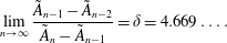 $$\begin{eqnarray}\lim _{n\rightarrow \infty }\frac{\tilde{A}_{n-1}-\tilde{A}_{n-2}}{\tilde{A}_{n}-\tilde{A}_{n-1}}=\unicode[STIX]{x1D6FF}=4.669\ldots .\end{eqnarray}$$
Recalling that the first bifurcation points are located at
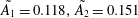 $\tilde{A_{1}}=0.118,\tilde{A_{2}}=0.151$
and
$\tilde{A_{1}}=0.118,\tilde{A_{2}}=0.151$
and
 $\tilde{A_{3}}=0.158$
(see also figure 12), we obtain
$\tilde{A_{3}}=0.158$
(see also figure 12), we obtain
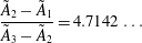 $$\begin{eqnarray}\frac{\tilde{A}_{2}-\tilde{A}_{1}}{\tilde{A}_{3}-\tilde{A}_{2}}=4.7142\ldots\end{eqnarray}$$
i.e. a value near the universal number
 $\unicode[STIX]{x1D6FF}$
found by Feigenbaum.
$\unicode[STIX]{x1D6FF}$
found by Feigenbaum.
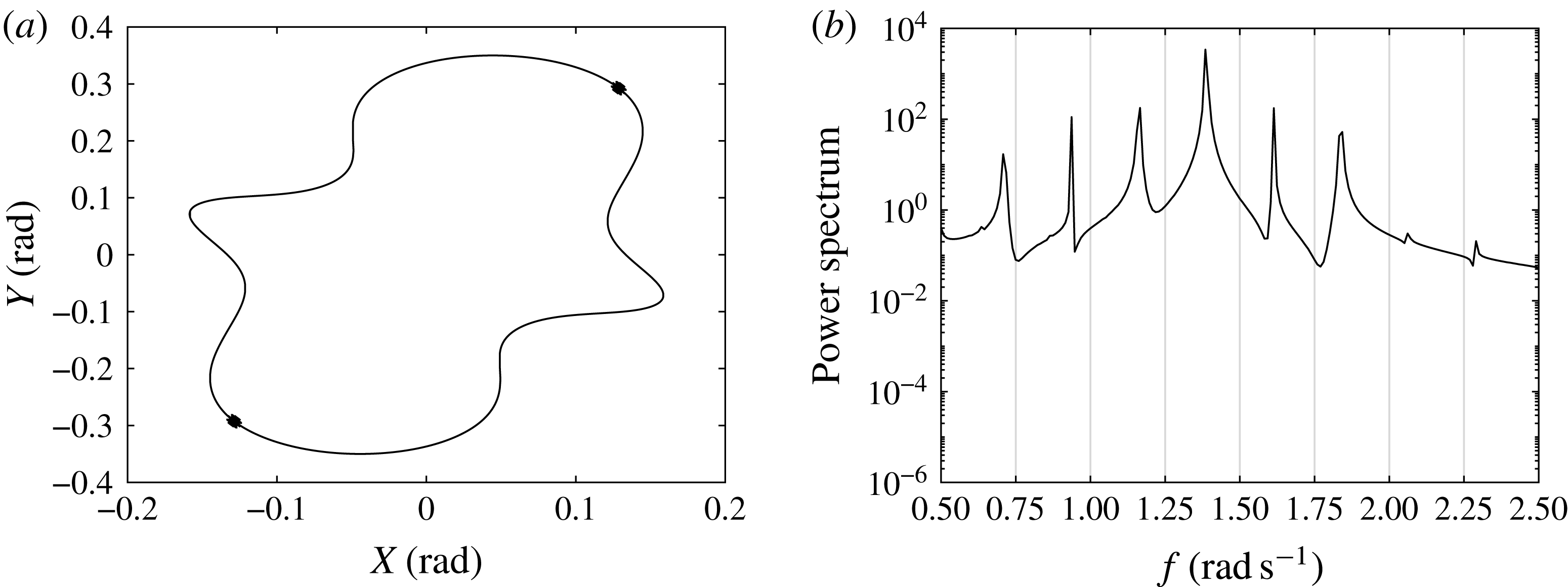
Figure 11. Period-two response and downshift at
 $\tilde{A}=0.25~\text{m}$
.
$\tilde{A}=0.25~\text{m}$
.
Figure 12. Period doubling scenarios as
 $\tilde{A}$
increases from 0 to 0.35 m.
$\tilde{A}$
increases from 0 to 0.35 m.
Finally we evaluate the effects of the chaotic response on the performance of the system. The incident wave amplitude is
 $\overline{A}+\tilde{A}\cos \unicode[STIX]{x1D6FA}t$
, hence the modulated incident wave potential
$\overline{A}+\tilde{A}\cos \unicode[STIX]{x1D6FA}t$
, hence the modulated incident wave potential
 $\unicode[STIX]{x1D6F7}_{m}^{I}$
is
$\unicode[STIX]{x1D6F7}_{m}^{I}$
is
 $$\begin{eqnarray}\unicode[STIX]{x1D6F7}_{m}^{I}=-\frac{\text{i}g(\overline{A}+\tilde{A}\cos \unicode[STIX]{x1D6FA}t)}{4\unicode[STIX]{x1D714}\cosh k_{0}h}\cosh k_{0}(h+z)\text{e}^{-\text{i}(k_{0}x+2\unicode[STIX]{x1D714}t)}+\ast ,\end{eqnarray}$$
and the corresponding averaged energy influx
 $$\begin{eqnarray}\lim _{\unicode[STIX]{x1D70F}\rightarrow \infty }-\frac{\unicode[STIX]{x1D70C}w}{\unicode[STIX]{x1D70F}}\int _{0}^{\unicode[STIX]{x1D70F}}\int _{-h}^{0}\unicode[STIX]{x1D6F7}_{m_{t}}^{I}\unicode[STIX]{x1D6F7}_{m_{x}}^{I}\,\text{d}z\,\text{d}t=\frac{\unicode[STIX]{x1D6FE}w\unicode[STIX]{x1D714}(2\overline{A}^{2}+\tilde{A})}{4k_{0}}\left(1+\frac{2k_{0}h}{2\sinh 2k_{0}h}\right).\end{eqnarray}$$
The averaged generated power by the array can be evaluated numerically by solving the following integral:
 $$\begin{eqnarray}P_{m}=\lim _{\unicode[STIX]{x1D70F}\rightarrow \infty }\frac{1}{\unicode[STIX]{x1D70F}}\int _{0}^{\unicode[STIX]{x1D70F}}(\unicode[STIX]{x1D6E9}_{t})^{2}\unicode[STIX]{x1D708}_{pto}\,\text{d}t.\end{eqnarray}$$
Figure 13 shows the capture factor of the array in modulated waves, defined as the ratio between
 $P_{m}$
(4.90) and the energy influx (4.89) for the same range of
$P_{m}$
(4.90) and the energy influx (4.89) for the same range of
 $\tilde{A}$
used before. Note that the minimum of the efficiency of the system is located in the range of
$\tilde{A}$
used before. Note that the minimum of the efficiency of the system is located in the range of
 $\tilde{A}$
where chaos occurs, while the maximum corresponds to
$\tilde{A}$
where chaos occurs, while the maximum corresponds to
 $\tilde{A}=0~\text{m}$
. When chaos disappears and regular motion returns with downshift,
$\tilde{A}=0~\text{m}$
. When chaos disappears and regular motion returns with downshift,
 ${\mathcal{C}}^{F}$
spikes to
${\mathcal{C}}^{F}$
spikes to
 ${\sim}0.2$
and starts again to decrease. In other words chaos and period doubling is detrimental in terms of wave energy extraction efficiency. We thus obtained a deterministic confirmation of the previous findings of Michele et al. (Reference Michele, Sammarco and d’Errico2016a
,Reference Michele, Sammarco and d’Errico
b
) for gate energy production under stochastic incident wave spectra. Finally, note that the value of the capture factor for
${\sim}0.2$
and starts again to decrease. In other words chaos and period doubling is detrimental in terms of wave energy extraction efficiency. We thus obtained a deterministic confirmation of the previous findings of Michele et al. (Reference Michele, Sammarco and d’Errico2016a
,Reference Michele, Sammarco and d’Errico
b
) for gate energy production under stochastic incident wave spectra. Finally, note that the value of the capture factor for
 $\tilde{A}=0$
m is
$\tilde{A}=0$
m is
 ${\mathcal{C}}^{F}\sim 0.35$
and corresponds to the same value shown in figure 6 for
${\mathcal{C}}^{F}\sim 0.35$
and corresponds to the same value shown in figure 6 for
 $\unicode[STIX]{x1D714}=3~\text{rad}~\text{s}^{-1}$
and uniform incident waves.
$\unicode[STIX]{x1D714}=3~\text{rad}~\text{s}^{-1}$
and uniform incident waves.
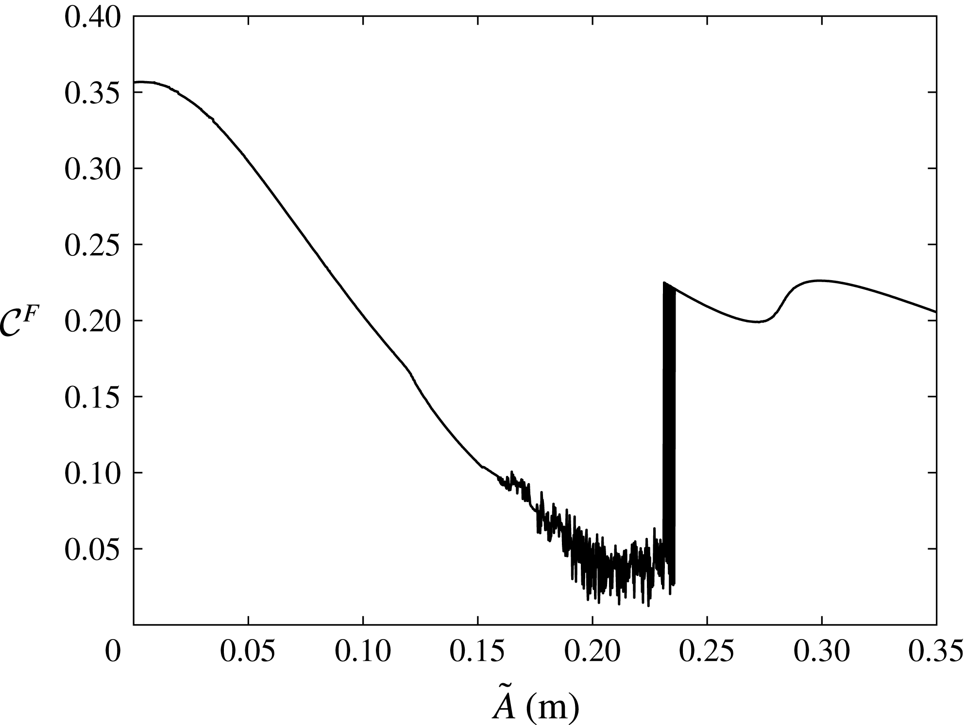
Figure 13. Behaviour of the capture factor of the array in modulated incident waves. Minima correspond to the range of
 $\tilde{A}$
where chaos occurs while the maximum is located at
$\tilde{A}$
where chaos occurs while the maximum is located at
 $\tilde{A}=0~\text{m}$
.
$\tilde{A}=0~\text{m}$
.
5 Resonance of two trapped modes by one incident wave
Let us assume the scales (2.2) and the presence at the leading order
 $O(1)$
of two natural modes having different eigenfrequencies
$O(1)$
of two natural modes having different eigenfrequencies
 $\unicode[STIX]{x1D714}_{1}$
and
$\unicode[STIX]{x1D714}_{1}$
and
 $\unicode[STIX]{x1D714}_{2}$
with
$\unicode[STIX]{x1D714}_{2}$
with
 $\unicode[STIX]{x1D714}_{2}>\unicode[STIX]{x1D714}_{1}$
. Quadratic interactions at
$\unicode[STIX]{x1D714}_{2}>\unicode[STIX]{x1D714}_{1}$
. Quadratic interactions at
 $O(\unicode[STIX]{x1D716})$
generates four harmonics, i.e.
$O(\unicode[STIX]{x1D716})$
generates four harmonics, i.e.
 $$\begin{eqnarray}2\unicode[STIX]{x1D714}_{1},2\unicode[STIX]{x1D714}_{2},(\unicode[STIX]{x1D714}_{1}+\unicode[STIX]{x1D714}_{2}),(\unicode[STIX]{x1D714}_{2}-\unicode[STIX]{x1D714}_{1}).\end{eqnarray}$$
Let the incident wave have the frequency
 $(\unicode[STIX]{x1D714}_{1}+\unicode[STIX]{x1D714}_{2})$
, the multiple-scale expansion of the potentials, free-surface elevation and mode amplitude are assumed as follows:
$(\unicode[STIX]{x1D714}_{1}+\unicode[STIX]{x1D714}_{2})$
, the multiple-scale expansion of the potentials, free-surface elevation and mode amplitude are assumed as follows:
 $$\begin{eqnarray}\displaystyle \unicode[STIX]{x1D6F7}^{\pm } & = & \displaystyle \unicode[STIX]{x1D719}_{11}^{\pm }(x,y,z,t_{2})\text{e}^{-\text{i}\unicode[STIX]{x1D714}_{1}t}+\unicode[STIX]{x1D719}_{12}^{\pm }(x,y,z,t_{2})\text{e}^{-\text{i}\unicode[STIX]{x1D714}_{2}t}\nonumber\\ \displaystyle & & \displaystyle +\,\unicode[STIX]{x1D716}[\!\unicode[STIX]{x1D719}_{21}^{\pm }(x,y,z,t_{2})\text{e}^{-2\text{i}\unicode[STIX]{x1D714}_{1}t}+\unicode[STIX]{x1D719}_{22}^{\pm }(x,y,z,t_{2})\text{e}^{-2\text{i}\unicode[STIX]{x1D714}_{2}t}+\unicode[STIX]{x1D719}_{23}^{\pm }(x,y,z,t_{2})\text{e}^{-\text{i}(\unicode[STIX]{x1D714}_{1}+\unicode[STIX]{x1D714}_{2})t}\nonumber\\ \displaystyle & & \displaystyle +\,\unicode[STIX]{x1D719}_{24}^{\pm }(x,y,z,t_{2})\text{e}^{-\text{i}(\unicode[STIX]{x1D714}_{2}-\unicode[STIX]{x1D714}_{1})t}\! ]+\,\unicode[STIX]{x1D716}^{2}[\unicode[STIX]{x1D719}_{31}^{\pm }(x,y,z,t_{2})\text{e}^{-\text{i}\unicode[STIX]{x1D714}_{1}t}+\unicode[STIX]{x1D719}_{32}^{\pm }(x,y,z,t_{2})\text{e}^{-\text{i}\unicode[STIX]{x1D714}_{2}t}]\qquad \nonumber\\ \displaystyle & & \displaystyle +\,\ast +O(\unicode[STIX]{x1D716}^{3}),\end{eqnarray}$$
 $$\begin{eqnarray}\displaystyle \unicode[STIX]{x1D701}^{\pm } & = & \displaystyle \unicode[STIX]{x1D701}_{11}^{\pm }(x,y,t_{2})\text{e}^{-\text{i}\unicode[STIX]{x1D714}_{1}t}+\unicode[STIX]{x1D701}_{12}^{\pm }(x,y,t_{2})\text{e}^{-\text{i}\unicode[STIX]{x1D714}_{2}t}\nonumber\\ \displaystyle & & \displaystyle +\,\unicode[STIX]{x1D716}[\!\unicode[STIX]{x1D701}_{21}^{\pm }(x,y,t_{2})\text{e}^{-2\text{i}\unicode[STIX]{x1D714}_{1}t}+\unicode[STIX]{x1D701}_{22}^{\pm }(x,y,t_{2})\text{e}^{-2\text{i}\unicode[STIX]{x1D714}_{2}t}+\unicode[STIX]{x1D701}_{23}^{\pm }(x,y,t_{2})\text{e}^{-\text{i}(\unicode[STIX]{x1D714}_{1}+\unicode[STIX]{x1D714}_{2})t}\nonumber\\ \displaystyle & & \displaystyle +\,\unicode[STIX]{x1D701}_{24}^{\pm }(x,y,t_{2})\text{e}^{-\text{i}(\unicode[STIX]{x1D714}_{2}-\unicode[STIX]{x1D714}_{1})t}\! ]+\,\unicode[STIX]{x1D716}^{2}[\unicode[STIX]{x1D701}_{31}^{\pm }(x,y,t_{2})\text{e}^{-\text{i}\unicode[STIX]{x1D714}_{1}t}+\unicode[STIX]{x1D701}_{32}^{\pm }(x,y,t_{2})\text{e}^{-\text{i}\unicode[STIX]{x1D714}_{2}t}]\nonumber\\ \displaystyle & & \displaystyle +\,\ast +O(\unicode[STIX]{x1D716}^{3}),\end{eqnarray}$$
 $$\begin{eqnarray}\displaystyle \unicode[STIX]{x1D6E9}^{\pm } & = & \displaystyle \unicode[STIX]{x1D703}_{11}(y,t_{2})\text{e}^{-\text{i}\unicode[STIX]{x1D714}_{1}t}+\unicode[STIX]{x1D703}_{12}(y,t_{2})\text{e}^{-\text{i}\unicode[STIX]{x1D714}_{2}t}\nonumber\\ \displaystyle & & \displaystyle +\,\unicode[STIX]{x1D716}[\!\unicode[STIX]{x1D703}_{21}(y,t_{2})\text{e}^{-2\text{i}\unicode[STIX]{x1D714}_{1}t}+\unicode[STIX]{x1D703}_{22}(y,t_{2})\text{e}^{-2\text{i}\unicode[STIX]{x1D714}_{2}t}+\unicode[STIX]{x1D703}_{23}(y,t_{2})\text{e}^{-\text{i}(\unicode[STIX]{x1D714}_{1}+\unicode[STIX]{x1D714}_{2})t}\nonumber\\ \displaystyle & & \displaystyle +\,\unicode[STIX]{x1D703}_{24}(y,t_{2})\text{e}^{-\text{i}(\unicode[STIX]{x1D714}_{2}-\unicode[STIX]{x1D714}_{1})t}\! ]+\,\unicode[STIX]{x1D716}^{2}[\unicode[STIX]{x1D703}_{31}(y,t_{2})\text{e}^{-\text{i}\unicode[STIX]{x1D714}_{1}t}+\unicode[STIX]{x1D703}_{32}(y,t_{2})\text{e}^{-\text{i}\unicode[STIX]{x1D714}_{2}t}]+\ast +O(\unicode[STIX]{x1D716}^{3}).\qquad\end{eqnarray}$$
5.1 Leading-order problem
$O(1)$

This is the same problem already explained in § 4.1. The solution consists of trapped modes whose related potentials
 $\unicode[STIX]{x1D719}_{11}$
,
$\unicode[STIX]{x1D719}_{11}$
,
 $\unicode[STIX]{x1D719}_{12}$
have the form
$\unicode[STIX]{x1D719}_{12}$
have the form
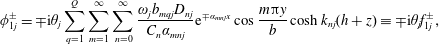 $$\begin{eqnarray}\unicode[STIX]{x1D719}_{1j}^{\pm }=\mp \text{i}\unicode[STIX]{x1D703}_{j}\mathop{\sum }_{q=1}^{Q}\mathop{\sum }_{m=1}^{\infty }\mathop{\sum }_{n=0}^{\infty }\frac{\unicode[STIX]{x1D714}_{j}b_{mqj}D_{nj}}{C_{n}\unicode[STIX]{x1D6FC}_{mnj}}\text{e}^{\mp \unicode[STIX]{x1D6FC}_{mnj}x}\cos \frac{m\unicode[STIX]{x03C0}y}{b}\cosh k_{nj}(h+z)\equiv \mp \text{i}\unicode[STIX]{x1D703}_{j}f_{1j}^{\pm },\end{eqnarray}$$
where the terms including the subscript
 $j=1,2$
, are relative to the
$j=1,2$
, are relative to the
 $j$
th mode with eigenfrequency
$j$
th mode with eigenfrequency
 $\unicode[STIX]{x1D714}_{j}$
and modal form
$\unicode[STIX]{x1D714}_{j}$
and modal form
 $\unicode[STIX]{x1D703}_{1j}=\{r_{1jq}\}\unicode[STIX]{x1D703}_{j}(t_{2})$
,
$\unicode[STIX]{x1D703}_{1j}=\{r_{1jq}\}\unicode[STIX]{x1D703}_{j}(t_{2})$
,
 $q=1,\ldots ,Q$
. To investigate the interactions between two modes it is necessary to consider the number of the gates
$q=1,\ldots ,Q$
. To investigate the interactions between two modes it is necessary to consider the number of the gates
 $Q>2$
because the number of trapped modes is
$Q>2$
because the number of trapped modes is
 $Q-1$
.
$Q-1$
.
5.2 The second-order problem
$O(\unicode[STIX]{x1D716})$

As mentioned before, let us assume at
 $O(1)$
the existence of a couple of trapped modes
$O(1)$
the existence of a couple of trapped modes
 $N_{1}$
and
$N_{1}$
and
 $N_{2}$
and the incident wave with frequency
$N_{2}$
and the incident wave with frequency
 $(\unicode[STIX]{x1D714}_{1}+\unicode[STIX]{x1D714}_{2})$
. At the order
$(\unicode[STIX]{x1D714}_{1}+\unicode[STIX]{x1D714}_{2})$
. At the order
 $O(\unicode[STIX]{x1D716})$
we have eight wave components generated by quadratic interactions of the
$O(\unicode[STIX]{x1D716})$
we have eight wave components generated by quadratic interactions of the
 $O(1)$
solution, i.e. the four harmonics (5.1) plus the respective complex conjugates.
$O(1)$
solution, i.e. the four harmonics (5.1) plus the respective complex conjugates.
We get the governing equation of each problem,
 $$\begin{eqnarray}\unicode[STIX]{x1D6FB}^{2}\unicode[STIX]{x1D719}_{2j}^{\pm }=0,\quad j=1,\ldots ,4,\end{eqnarray}$$
the relative boundary conditions on the moving gates,
 $$\begin{eqnarray}\displaystyle & \displaystyle \unicode[STIX]{x1D719}_{21_{x}}^{\pm }=\left[2\text{i}\unicode[STIX]{x1D714}_{1}\unicode[STIX]{x1D703}_{21}(z+h_{p})-\frac{\unicode[STIX]{x1D719}_{1_{z}}^{\pm }\unicode[STIX]{x1D703}_{1}}{\unicode[STIX]{x1D716}}\mp \text{i}\unicode[STIX]{x1D714}_{1}\,d\frac{\unicode[STIX]{x1D703}_{1}^{2}}{\unicode[STIX]{x1D716}}\right]H(z+h-c), & \displaystyle\end{eqnarray}$$
 $$\begin{eqnarray}\displaystyle & \displaystyle \unicode[STIX]{x1D719}_{22_{x}}^{\pm }=\left[2\text{i}\unicode[STIX]{x1D714}_{2}\unicode[STIX]{x1D703}_{22}(z+h_{p})-\frac{\unicode[STIX]{x1D719}_{2_{z}}^{\pm }\unicode[STIX]{x1D703}_{2}}{\unicode[STIX]{x1D716}}\mp \text{i}\unicode[STIX]{x1D714}_{2}\,d\frac{\unicode[STIX]{x1D703}_{2}^{2}}{\unicode[STIX]{x1D716}}\right]H(z+h-c), & \displaystyle\end{eqnarray}$$
 $$\begin{eqnarray}\displaystyle \unicode[STIX]{x1D719}_{23_{x}}^{\pm } & = & \displaystyle \left[\text{i}(\unicode[STIX]{x1D714}_{1}+\unicode[STIX]{x1D714}_{2})\unicode[STIX]{x1D703}_{23}(z+h_{p})-\frac{\unicode[STIX]{x1D719}_{2_{z}}^{\pm }\unicode[STIX]{x1D703}_{1}+\unicode[STIX]{x1D719}_{1_{z}}^{\pm }\unicode[STIX]{x1D703}_{2}}{\unicode[STIX]{x1D716}}\right.\nonumber\\ \displaystyle & & \displaystyle \left.\mp \,\text{i}d(\unicode[STIX]{x1D714}_{1}+\unicode[STIX]{x1D714}_{2})\frac{\unicode[STIX]{x1D703}_{1}\unicode[STIX]{x1D703}_{2}}{\unicode[STIX]{x1D716}}\right]H(z+h-c),\end{eqnarray}$$
 $$\begin{eqnarray}\displaystyle \unicode[STIX]{x1D719}_{24_{x}}^{\pm } & = & \displaystyle \left[\text{i}(\unicode[STIX]{x1D714}_{2}-\unicode[STIX]{x1D714}_{1})\unicode[STIX]{x1D703}_{24}(z+h_{p})-\frac{\unicode[STIX]{x1D719}_{2_{z}}^{\pm }\unicode[STIX]{x1D703}_{1}^{\ast }+\unicode[STIX]{x1D719}_{1_{z}}^{\pm ^{\ast }}\unicode[STIX]{x1D703}_{2}}{\unicode[STIX]{x1D716}}\right.\nonumber\\ \displaystyle & & \displaystyle \left.\mp \,\text{i}d(\unicode[STIX]{x1D714}_{2}-\unicode[STIX]{x1D714}_{1})\frac{\unicode[STIX]{x1D703}_{1}^{\ast }\unicode[STIX]{x1D703}_{2}}{\unicode[STIX]{x1D716}}\right]H(z+h-c),\quad x=x^{\pm },\end{eqnarray}$$
the mixed boundary conditions on the free surface,
 $$\begin{eqnarray}\displaystyle & \displaystyle \unicode[STIX]{x1D719}_{21_{z}}^{\pm }=\unicode[STIX]{x1D719}_{21}^{\pm }\frac{4\unicode[STIX]{x1D714}_{1}^{2}}{g}, & \displaystyle\end{eqnarray}$$
 $$\begin{eqnarray}\displaystyle & \displaystyle \unicode[STIX]{x1D719}_{22_{z}}^{\pm }=\unicode[STIX]{x1D719}_{22}^{\pm }\frac{4\unicode[STIX]{x1D714}_{2}^{2}}{g}, & \displaystyle\end{eqnarray}$$
 $$\begin{eqnarray}\displaystyle & \displaystyle \unicode[STIX]{x1D719}_{23_{z}}^{\pm }=\unicode[STIX]{x1D719}_{23}^{\pm }\frac{(\unicode[STIX]{x1D714}_{1}+\unicode[STIX]{x1D714}_{2})^{2}}{g}, & \displaystyle\end{eqnarray}$$
 $$\begin{eqnarray}\displaystyle & \displaystyle \unicode[STIX]{x1D719}_{24_{z}}^{\pm }=\unicode[STIX]{x1D719}_{24}^{\pm }\frac{(\unicode[STIX]{x1D714}_{2}-\unicode[STIX]{x1D714}_{1})^{2}}{g},\quad z=0, & \displaystyle\end{eqnarray}$$
and the corresponding free-surface elevations,
 $$\begin{eqnarray}\displaystyle & \displaystyle \unicode[STIX]{x1D702}_{21}^{\pm }=\frac{2\text{i}\unicode[STIX]{x1D714}_{1}}{g}\unicode[STIX]{x1D719}_{21}^{\pm }, & \displaystyle\end{eqnarray}$$
 $$\begin{eqnarray}\displaystyle & \displaystyle \unicode[STIX]{x1D702}_{22}^{\pm }=\frac{2\text{i}\unicode[STIX]{x1D714}_{2}}{g}\unicode[STIX]{x1D719}_{22}^{\pm }, & \displaystyle\end{eqnarray}$$
 $$\begin{eqnarray}\displaystyle & \displaystyle \unicode[STIX]{x1D702}_{23}^{\pm }=\frac{\text{i}(\unicode[STIX]{x1D714}_{1}+\unicode[STIX]{x1D714}_{2})}{g}\unicode[STIX]{x1D719}_{23}^{\pm }, & \displaystyle\end{eqnarray}$$
 $$\begin{eqnarray}\displaystyle & \displaystyle \unicode[STIX]{x1D702}_{24}^{\pm }=\frac{\text{i}(\unicode[STIX]{x1D714}_{2}-\unicode[STIX]{x1D714}_{1})}{g}\unicode[STIX]{x1D719}_{24}^{\pm },\quad z=0. & \displaystyle\end{eqnarray}$$
As in § 4.2, we obtain the second-order solution of each
 $j$
th wave field component,
$j$
th wave field component,
 $$\begin{eqnarray}\unicode[STIX]{x1D719}_{2j}^{\pm }=\tilde{\unicode[STIX]{x1D703}}_{j}\mathop{\sum }_{p=0}^{\infty }\mathop{\sum }_{l=0}^{\infty }\frac{\unicode[STIX]{x1D6E5}_{plj}}{\unicode[STIX]{x1D6FC}_{plj}\unicode[STIX]{x1D716}}\text{e}^{\pm \text{i}\unicode[STIX]{x1D6FC}_{plj}x}\cos \frac{p\unicode[STIX]{x03C0}y}{b}\cosh k_{lj}(h+z),\quad j=1,\ldots ,4,\end{eqnarray}$$
where
 $\tilde{\unicode[STIX]{x1D703}}(t)=\{\unicode[STIX]{x1D703}_{1}^{2},\unicode[STIX]{x1D703}_{2}^{2},\unicode[STIX]{x1D703}_{1}\unicode[STIX]{x1D703}_{2},\unicode[STIX]{x1D703}_{1}\unicode[STIX]{x1D703}_{2}^{\ast }\}$
is the vector that contains the combinations of the resonated mode amplitudes,
$\tilde{\unicode[STIX]{x1D703}}(t)=\{\unicode[STIX]{x1D703}_{1}^{2},\unicode[STIX]{x1D703}_{2}^{2},\unicode[STIX]{x1D703}_{1}\unicode[STIX]{x1D703}_{2},\unicode[STIX]{x1D703}_{1}\unicode[STIX]{x1D703}_{2}^{\ast }\}$
is the vector that contains the combinations of the resonated mode amplitudes,
 $k_{lj}$
are the roots of the dispersion relations,
$k_{lj}$
are the roots of the dispersion relations,
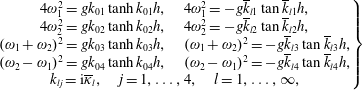 $$\begin{eqnarray}\left.\begin{array}{@{}c@{}}4\unicode[STIX]{x1D714}_{1}^{2}=gk_{01}\tanh k_{01}h,\quad 4\unicode[STIX]{x1D714}_{1}^{2}=-g\overline{k}_{l1}\tan \overline{k}_{l1}h,\\ 4\unicode[STIX]{x1D714}_{2}^{2}=gk_{02}\tanh k_{02}h,\quad 4\unicode[STIX]{x1D714}_{2}^{2}=-g\overline{k}_{l2}\tan \overline{k}_{l2}h,\\ (\unicode[STIX]{x1D714}_{1}+\unicode[STIX]{x1D714}_{2})^{2}=gk_{03}\tanh k_{03}h,\quad (\unicode[STIX]{x1D714}_{1}+\unicode[STIX]{x1D714}_{2})^{2}=-g\overline{k}_{l3}\tan \overline{k}_{l3}h,\\ (\unicode[STIX]{x1D714}_{2}-\unicode[STIX]{x1D714}_{1})^{2}=gk_{04}\tanh k_{04}h,\quad (\unicode[STIX]{x1D714}_{2}-\unicode[STIX]{x1D714}_{1})^{2}=-g\overline{k}_{l4}\tan \overline{k}_{l4}h,\\ k_{lj}=\text{i}\overline{\unicode[STIX]{x1D705}}_{l},\quad j=1,\ldots ,4,\quad l=1,\ldots ,\infty ,\end{array}\right\}\end{eqnarray}$$
while
 $\unicode[STIX]{x1D6E5}_{plj}$
is a complex coefficient evaluated in appendix A. Similarly to the previous case, the gate motion at this order is null (
$\unicode[STIX]{x1D6E5}_{plj}$
is a complex coefficient evaluated in appendix A. Similarly to the previous case, the gate motion at this order is null (
 $\unicode[STIX]{x1D703}_{2j}=0$
,
$\unicode[STIX]{x1D703}_{2j}=0$
,
 $j=1,\ldots ,4$
), however there are propagating waves that radiate energy to infinity and damp mode motion through cubic interactions at the third order.
$j=1,\ldots ,4$
), however there are propagating waves that radiate energy to infinity and damp mode motion through cubic interactions at the third order.
5.3 The coupled evolution equations
At this order we apply the solvability condition which is found by Green’s formula:
 $$\begin{eqnarray}\displaystyle 0 & = & \displaystyle \frac{\unicode[STIX]{x1D714}_{j}^{2}}{g}\int _{0}^{b}\,\text{d}y\left(\int _{-\infty }^{0}f_{1j}^{-}{\mathcal{F}}_{3j}^{-}\,\text{d}x-\int _{0}^{\infty }f_{1j}^{+}{\mathcal{F}}_{3j}^{+}\,\text{d}x\right)\nonumber\\ \displaystyle & & \displaystyle +\,2\int _{0}^{b}\,\text{d}y\int _{-h}^{0}\overline{f_{j}{\mathcal{G}}_{3j}}\,\text{d}z+\mathop{\sum }_{q=1}^{Q}\left(\frac{\text{i}{\mathcal{D}}_{3j}r_{1jq}}{\unicode[STIX]{x1D70C}}-\frac{\unicode[STIX]{x1D708}_{pto}r_{1jq}^{2}\unicode[STIX]{x1D714}_{j}\unicode[STIX]{x1D703}_{j}}{\unicode[STIX]{x1D70C}\unicode[STIX]{x1D716}^{2}}\right),\quad j=1,2.\end{eqnarray}$$
Details of the forcing terms in the latter equation can be found in appendix B. Carrying out the integrals of (5.21) and grouping the terms according to
 $\unicode[STIX]{x1D703}_{11}$
,
$\unicode[STIX]{x1D703}_{11}$
,
 $\unicode[STIX]{x1D703}_{12}$
,
$\unicode[STIX]{x1D703}_{12}$
,
 $\unicode[STIX]{x1D703}_{11}\left|\unicode[STIX]{x1D703}_{11}\right|^{2}$
,
$\unicode[STIX]{x1D703}_{11}\left|\unicode[STIX]{x1D703}_{11}\right|^{2}$
,
 $\unicode[STIX]{x1D703}_{11}\left|\unicode[STIX]{x1D703}_{12}\right|^{2}$
,
$\unicode[STIX]{x1D703}_{11}\left|\unicode[STIX]{x1D703}_{12}\right|^{2}$
,
 $\unicode[STIX]{x1D703}_{12}\left|\unicode[STIX]{x1D703}_{12}\right|^{2}$
,
$\unicode[STIX]{x1D703}_{12}\left|\unicode[STIX]{x1D703}_{12}\right|^{2}$
,
 $\unicode[STIX]{x1D703}_{12}\left|\unicode[STIX]{x1D703}_{11}\right|^{2}$
,
$\unicode[STIX]{x1D703}_{12}\left|\unicode[STIX]{x1D703}_{11}\right|^{2}$
,
 $\unicode[STIX]{x1D703}_{11}^{\ast }$
,
$\unicode[STIX]{x1D703}_{11}^{\ast }$
,
 $\unicode[STIX]{x1D703}_{12}^{\ast }$
, we obtain two coupled evolution equations for both modal oscillations
$\unicode[STIX]{x1D703}_{12}^{\ast }$
, we obtain two coupled evolution equations for both modal oscillations
 $\unicode[STIX]{x1D703}_{11}$
and
$\unicode[STIX]{x1D703}_{11}$
and
 $\unicode[STIX]{x1D703}_{12}$
:
$\unicode[STIX]{x1D703}_{12}$
:
 $$\begin{eqnarray}\displaystyle & \displaystyle -\text{i}\unicode[STIX]{x1D703}_{11_{t}}=\unicode[STIX]{x1D703}_{11}|\unicode[STIX]{x1D703}_{11}|^{2}(c_{N}+\text{i}c_{R})+\unicode[STIX]{x1D703}_{11}|\unicode[STIX]{x1D703}_{12}|^{2}(c_{S}+\text{i}c_{U})+A\unicode[STIX]{x1D703}_{12}^{\ast }c_{F}+\text{i}\unicode[STIX]{x1D703}_{11}\unicode[STIX]{x1D708}_{pto}c_{L}, & \displaystyle\end{eqnarray}$$
 $$\begin{eqnarray}\displaystyle & \displaystyle -\text{i}\unicode[STIX]{x1D703}_{12_{t}}=\unicode[STIX]{x1D703}_{12}|\unicode[STIX]{x1D703}_{12}|^{2}(d_{N}+\text{i}d_{R})+\unicode[STIX]{x1D703}_{12}|\unicode[STIX]{x1D703}_{11}|^{2}(d_{S}+\text{i}d_{U})+A\unicode[STIX]{x1D703}_{11}^{\ast }d_{F}+\text{i}\unicode[STIX]{x1D703}_{12}\unicode[STIX]{x1D708}_{pto}d_{L}, & \displaystyle\end{eqnarray}$$
where the coupling coefficients are evaluated in a similar manner as explained in § 4.3. Differently to the case of single-mode subharmonic excitation we have two new pairs of coefficients as in the edge wave theories,
 $c_{S},d_{S},c_{U},d_{U}$
, that represent the coupling between the modes. Note also that in (5.22) the incident wave amplitude
$c_{S},d_{S},c_{U},d_{U}$
, that represent the coupling between the modes. Note also that in (5.22) the incident wave amplitude
 $A$
is multiplied by the complex conjugate of
$A$
is multiplied by the complex conjugate of
 $\unicode[STIX]{x1D703}_{12}$
, while in (5.23) the same term is multiplied by
$\unicode[STIX]{x1D703}_{12}$
, while in (5.23) the same term is multiplied by
 $\unicode[STIX]{x1D703}_{11}^{\ast }$
. This depends on the fact that the incident wave frequency is assumed to be equal to
$\unicode[STIX]{x1D703}_{11}^{\ast }$
. This depends on the fact that the incident wave frequency is assumed to be equal to
 $\left(\unicode[STIX]{x1D714}_{1}+\unicode[STIX]{x1D714}_{2}\right)$
and not equal to twice the eigenfrequency of a single mode. Now consider the detuning of the incident wave frequency
$\left(\unicode[STIX]{x1D714}_{1}+\unicode[STIX]{x1D714}_{2}\right)$
and not equal to twice the eigenfrequency of a single mode. Now consider the detuning of the incident wave frequency
 $\unicode[STIX]{x0394}\unicode[STIX]{x1D714}$
with
$\unicode[STIX]{x0394}\unicode[STIX]{x1D714}$
with
 $\unicode[STIX]{x0394}\unicode[STIX]{x1D714}/\unicode[STIX]{x1D714}\sim O(\unicode[STIX]{x1D716}^{2})$
and let us assume the following change of variables:
$\unicode[STIX]{x0394}\unicode[STIX]{x1D714}/\unicode[STIX]{x1D714}\sim O(\unicode[STIX]{x1D716}^{2})$
and let us assume the following change of variables:
 $$\begin{eqnarray}\unicode[STIX]{x1D703}_{j}=\overline{\unicode[STIX]{x1D703}}_{j}\text{e}^{-\text{i}\unicode[STIX]{x0394}\unicode[STIX]{x1D714}_{j}t},\quad j=1,2,\end{eqnarray}$$
where
 $\unicode[STIX]{x0394}\unicode[STIX]{x1D714}=\unicode[STIX]{x0394}\unicode[STIX]{x1D714}_{1}+\unicode[STIX]{x0394}\unicode[STIX]{x1D714}_{2}$
. Then the evolution equations modify as follows:
$\unicode[STIX]{x0394}\unicode[STIX]{x1D714}=\unicode[STIX]{x0394}\unicode[STIX]{x1D714}_{1}+\unicode[STIX]{x0394}\unicode[STIX]{x1D714}_{2}$
. Then the evolution equations modify as follows:
 $$\begin{eqnarray}\displaystyle & \displaystyle -\text{i}\overline{\unicode[STIX]{x1D703}}_{11_{t}}=\unicode[STIX]{x0394}\unicode[STIX]{x1D714}_{1}\overline{\unicode[STIX]{x1D703}}_{11}+\overline{\unicode[STIX]{x1D703}}_{11}|\overline{\unicode[STIX]{x1D703}}_{11}|^{2}(c_{N}+\text{i}c_{R})+\overline{\unicode[STIX]{x1D703}}_{11}|\overline{\unicode[STIX]{x1D703}}_{12}|^{2}(c_{S}+\text{i}c_{U})+A\overline{\unicode[STIX]{x1D703}}_{12}^{\ast }c_{F}+\text{i}\overline{\unicode[STIX]{x1D703}}_{11}\unicode[STIX]{x1D708}_{pto}c_{L}, & \displaystyle \nonumber\\ \displaystyle & & \displaystyle\end{eqnarray}$$
 $$\begin{eqnarray}\displaystyle & \displaystyle -\text{i}\overline{\unicode[STIX]{x1D703}}_{12_{t}}=\unicode[STIX]{x0394}\unicode[STIX]{x1D714}_{2}\overline{\unicode[STIX]{x1D703}}_{12}+\overline{\unicode[STIX]{x1D703}}_{12}|\overline{\unicode[STIX]{x1D703}}_{12}|^{2}(d_{N}+\text{i}d_{R})+\overline{\unicode[STIX]{x1D703}}_{12}|\overline{\unicode[STIX]{x1D703}}_{11}|^{2}(d_{S}+\text{i}d_{U})+A\overline{\unicode[STIX]{x1D703}}_{11}^{\ast }d_{F}+\text{i}\overline{\unicode[STIX]{x1D703}}_{12}\unicode[STIX]{x1D708}_{pto}d_{L}. & \displaystyle \nonumber\\ \displaystyle & & \displaystyle\end{eqnarray}$$
5.4 Analysis of the coupled equations and theoretical results
Consider an array of
 $Q=4$
gates with characteristics listed in table 3. We obtain two odd natural modes and a single even mode (see also Sammarco et al.
Reference Sammarco, Michele and d’Errico2013). Interaction between odd–even modes yields the coefficients
$Q=4$
gates with characteristics listed in table 3. We obtain two odd natural modes and a single even mode (see also Sammarco et al.
Reference Sammarco, Michele and d’Errico2013). Interaction between odd–even modes yields the coefficients
 $c_{F},d_{F}$
equal to zero and the system of (5.25)–(5.26) becomes unforced. As a consequence, we can consider the interaction between the odd modes only, with shape
$c_{F},d_{F}$
equal to zero and the system of (5.25)–(5.26) becomes unforced. As a consequence, we can consider the interaction between the odd modes only, with shape
 $r_{11q}=\{1,0.41,-0.41,-1\}$
and
$r_{11q}=\{1,0.41,-0.41,-1\}$
and
 $r_{12q}=\{1,-2.41,2.41,-1\}$
. Sample values of the coefficients of (5.25)–(5.26) are shown in figure 14. Note that
$r_{12q}=\{1,-2.41,2.41,-1\}$
. Sample values of the coefficients of (5.25)–(5.26) are shown in figure 14. Note that
 $c_{U}$
and
$c_{U}$
and
 $d_{U}$
(figure 14
e) are very small if compared to the others and tend to increase for large eigenfrequencies while
$d_{U}$
(figure 14
e) are very small if compared to the others and tend to increase for large eigenfrequencies while
 $c_{F}$
is larger than
$c_{F}$
is larger than
 $d_{F}$
although
$d_{F}$
although
 $\unicode[STIX]{x1D714}_{1}<\unicode[STIX]{x1D714}_{2}$
for fixed gate characteristics. This has an important consequence because
$\unicode[STIX]{x1D714}_{1}<\unicode[STIX]{x1D714}_{2}$
for fixed gate characteristics. This has an important consequence because
 $N_{1}$
can be forced more easily by the incident waves.
$N_{1}$
can be forced more easily by the incident waves.
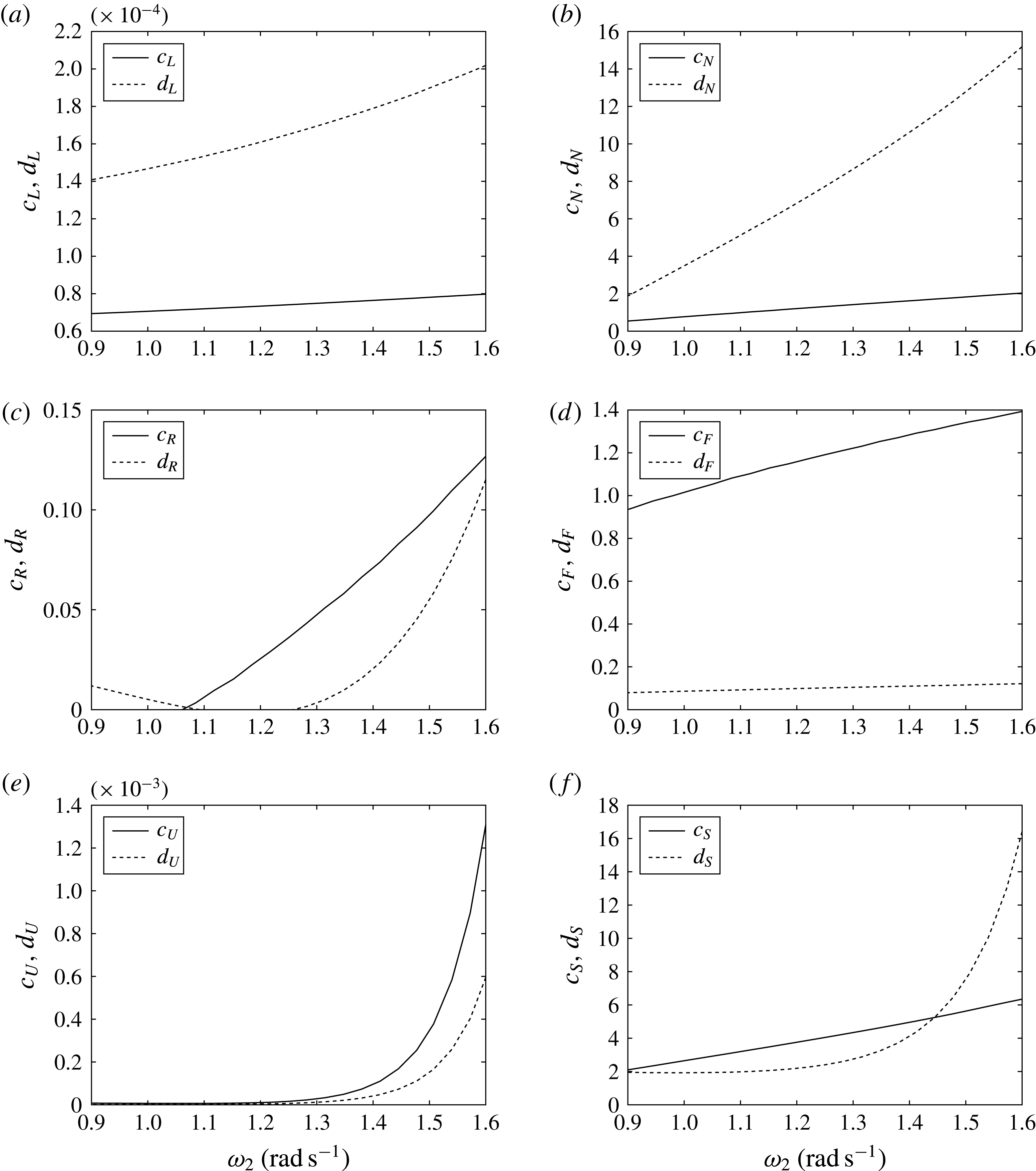
Figure 14. Behaviour of the coefficients of the evolution equations versus the eigenfrequency of the mode
 $N_{2}$
,
$N_{2}$
,
 $\unicode[STIX]{x1D714}_{2}$
.
$\unicode[STIX]{x1D714}_{2}$
.
Now define
 $\overline{\unicode[STIX]{x1D703}}_{1j}$
in action-angle variables form, i.e.
$\overline{\unicode[STIX]{x1D703}}_{1j}$
in action-angle variables form, i.e.
 $\overline{\unicode[STIX]{x1D703}}_{1j}=\text{i}\sqrt{R_{j}}\text{e}^{\text{i}\unicode[STIX]{x1D713}_{j}}$
, and neglect
$\overline{\unicode[STIX]{x1D703}}_{1j}=\text{i}\sqrt{R_{j}}\text{e}^{\text{i}\unicode[STIX]{x1D713}_{j}}$
, and neglect
 $c_{U},d_{U}$
with respect to the other coefficients to reduce the algebra without simplifying the physics. Then, from (5.25)–(5.26), we obtain a system of four real differential equations:
$c_{U},d_{U}$
with respect to the other coefficients to reduce the algebra without simplifying the physics. Then, from (5.25)–(5.26), we obtain a system of four real differential equations:
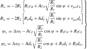 $$\begin{eqnarray}\left.\begin{array}{@{}c@{}}\displaystyle R_{1_{t}}=-2R_{1}\left[R_{1}c_{R}+Ac_{F}\sqrt{\frac{R_{2}}{R_{1}}}\sin \unicode[STIX]{x1D713}+\unicode[STIX]{x1D708}_{pto}c_{L}\right]\\ \displaystyle R_{2_{t}}=-2R_{2}\left[R_{2}d_{R}+Ad_{F}\sqrt{\frac{R_{1}}{R_{2}}}\sin \unicode[STIX]{x1D713}+\unicode[STIX]{x1D708}_{pto}d_{L}\right]\\ \displaystyle \unicode[STIX]{x1D713}_{1_{t}}=\unicode[STIX]{x0394}\unicode[STIX]{x1D714}_{1}-Ac_{F}\sqrt{\frac{R_{2}}{R_{1}}}\cos \unicode[STIX]{x1D713}+R_{1}c_{N}+R_{2}c_{S}\\ \displaystyle \unicode[STIX]{x1D713}_{2_{t}}=\unicode[STIX]{x0394}\unicode[STIX]{x1D714}_{2}-Ad_{F}\sqrt{\frac{R_{1}}{R_{2}}}\cos \unicode[STIX]{x1D713}+R_{1}d_{S}+R_{2}d_{N},\end{array}\right\}\end{eqnarray}$$
in which
 $\unicode[STIX]{x1D713}=\unicode[STIX]{x1D713}_{1}+\unicode[STIX]{x1D713}_{2}$
denotes the sum of the modal phases. After a long time the system reaches equilibrium, hence we now focus our attention on determining the fixed points of (5.27). The trivial fixed point is at
$\unicode[STIX]{x1D713}=\unicode[STIX]{x1D713}_{1}+\unicode[STIX]{x1D713}_{2}$
denotes the sum of the modal phases. After a long time the system reaches equilibrium, hence we now focus our attention on determining the fixed points of (5.27). The trivial fixed point is at
 $$\begin{eqnarray}R_{1}=R_{2}=0,\quad \unicode[STIX]{x1D713}^{\ast }=\cos ^{-1}\frac{\unicode[STIX]{x0394}\unicode[STIX]{x1D714}}{A(c_{F}+d_{F})},\end{eqnarray}$$
while non-trivial fixed points related to unstable and stable equilibria correspond to the roots of the system
 $$\begin{eqnarray}R_{2}=\frac{1}{2d_{R}}\left[-\unicode[STIX]{x1D708}_{pto}d_{L}+\sqrt{\unicode[STIX]{x1D708}_{pto}^{2}d_{L}^{2}+\frac{4d_{F}d_{R}R_{1}(\unicode[STIX]{x1D708}_{pto}c_{L}+c_{R}R_{1})}{c_{F}}}\right],\end{eqnarray}$$
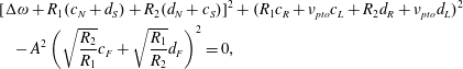 $$\begin{eqnarray}\displaystyle & & \displaystyle [\unicode[STIX]{x0394}\unicode[STIX]{x1D714}+R_{1}(c_{N}+d_{S})+R_{2}(d_{N}+c_{S})]^{2}+(R_{1}c_{R}+\unicode[STIX]{x1D708}_{pto}c_{L}+R_{2}d_{R}+\unicode[STIX]{x1D708}_{pto}d_{L})^{2}\nonumber\\ \displaystyle & & \displaystyle \quad -\,A^{2}\left(\sqrt{\frac{R_{2}}{R_{1}}}c_{F}+\sqrt{\frac{R_{1}}{R_{2}}}d_{F}\right)^{2}=0,\end{eqnarray}$$
which can be found numerically. Note that if
 $R_{1}=0$
also
$R_{1}=0$
also
 $R_{2}=0$
and triad resonance does not occur. Stability analysis of the linearized system (5.25)–(5.26) at the origin allows us to find the threshold of resonance triad,
$R_{2}=0$
and triad resonance does not occur. Stability analysis of the linearized system (5.25)–(5.26) at the origin allows us to find the threshold of resonance triad,
 $$\begin{eqnarray}A>\unicode[STIX]{x1D708}_{pto}\sqrt{\frac{c_{L}d_{L}}{c_{F}d_{F}}},\end{eqnarray}$$
hence the amplitude of the incident wave must be larger than the latter quantity to trigger mode–mode interactions. Once the equilibrium states
 $R_{1}$
and
$R_{1}$
and
 $R_{2}$
are evaluated we determine the sum of the modal phases by manipulating
$R_{2}$
are evaluated we determine the sum of the modal phases by manipulating
 $\unicode[STIX]{x1D713}_{1_{t}}$
and
$\unicode[STIX]{x1D713}_{1_{t}}$
and
 $\unicode[STIX]{x1D713}_{2_{t}}$
:
$\unicode[STIX]{x1D713}_{2_{t}}$
:
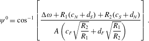 $$\begin{eqnarray}\unicode[STIX]{x1D713}^{0}=\cos ^{-1}\left[\frac{\unicode[STIX]{x0394}\unicode[STIX]{x1D714}+R_{1}(c_{N}+d_{S})+R_{2}(c_{S}+d_{N})}{A\displaystyle \left(c_{F}\sqrt{\frac{R_{2}}{R_{1}}}+d_{F}\sqrt{\frac{R_{1}}{R_{2}}}\right)}\right].\end{eqnarray}$$
Substitution of
 $\unicode[STIX]{x1D713}=\unicode[STIX]{x1D713}^{0}$
inside (5.27) gives
$\unicode[STIX]{x1D713}=\unicode[STIX]{x1D713}^{0}$
inside (5.27) gives
 $\unicode[STIX]{x0394}\unicode[STIX]{x1D714}_{1}$
and
$\unicode[STIX]{x0394}\unicode[STIX]{x1D714}_{1}$
and
 $\unicode[STIX]{x0394}\unicode[STIX]{x1D714}_{2}$
. Physically, the latter terms are the speed along the limit cycles in the complex plane
$\unicode[STIX]{x0394}\unicode[STIX]{x1D714}_{2}$
. Physically, the latter terms are the speed along the limit cycles in the complex plane
 $\text{Re}\{\unicode[STIX]{x1D703}\},\text{Im}\{\unicode[STIX]{x1D703}\}$
. The generated power due to triad resonance is finally given by
$\text{Re}\{\unicode[STIX]{x1D703}\},\text{Im}\{\unicode[STIX]{x1D703}\}$
. The generated power due to triad resonance is finally given by
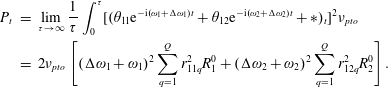 $$\begin{eqnarray}\displaystyle P_{t} & = & \displaystyle \lim _{\unicode[STIX]{x1D70F}\rightarrow \infty }\frac{1}{\unicode[STIX]{x1D70F}}\int _{0}^{\unicode[STIX]{x1D70F}}[(\unicode[STIX]{x1D703}_{11}\text{e}^{-\text{i}(\unicode[STIX]{x1D714}_{1}+\unicode[STIX]{x0394}\unicode[STIX]{x1D714}_{1})t}+\unicode[STIX]{x1D703}_{12}\text{e}^{-\text{i}(\unicode[STIX]{x1D714}_{2}+\unicode[STIX]{x0394}\unicode[STIX]{x1D714}_{2})t}+\ast )_{t}]^{2}\unicode[STIX]{x1D708}_{pto}\nonumber\\ \displaystyle & = & \displaystyle 2\unicode[STIX]{x1D708}_{pto}\left[(\unicode[STIX]{x0394}\unicode[STIX]{x1D714}_{1}+\unicode[STIX]{x1D714}_{1})^{2}\mathop{\sum }_{q=1}^{Q}r_{11q}^{2}R_{1}^{0}+(\unicode[STIX]{x0394}\unicode[STIX]{x1D714}_{2}+\unicode[STIX]{x1D714}_{2})^{2}\mathop{\sum }_{q=1}^{Q}r_{12q}^{2}R_{2}^{0}\right].\end{eqnarray}$$
Now focus the attention on a fixed OWSC configuration and analyse the effects of triad resonance on the performances of the array. Let us consider the case where the system has the eigenfrequency
 $\unicode[STIX]{x1D714}_{2}=1.5~\text{rad}~\text{s}^{-1}$
. Solution of the eigenvalue condition at the first order gives the eigenfrequency of the mode
$\unicode[STIX]{x1D714}_{2}=1.5~\text{rad}~\text{s}^{-1}$
. Solution of the eigenvalue condition at the first order gives the eigenfrequency of the mode
 $N_{1}$
, i.e.
$N_{1}$
, i.e.
 $\unicode[STIX]{x1D714}_{1}=0.9~\text{rad}~\text{s}^{-1}$
. The corresponding evolution equation coefficients are (see also figure 14):
$\unicode[STIX]{x1D714}_{1}=0.9~\text{rad}~\text{s}^{-1}$
. The corresponding evolution equation coefficients are (see also figure 14):
 $$\begin{eqnarray}\left.\begin{array}{@{}c@{}}c_{N}=1.84,\quad c_{R}=0.1,\quad c_{F}=1.34,\quad c_{S}=5.68,\\ d_{N}=12.96,\quad d_{R}=0.06,\quad d_{F}=0.11,\quad d_{S}=7.93.\end{array}\right\}\end{eqnarray}$$
Choose the
 $\unicode[STIX]{x1D708}_{pto}$
which maximizes power output for perfect resonance, i.e.
$\unicode[STIX]{x1D708}_{pto}$
which maximizes power output for perfect resonance, i.e.
 $\unicode[STIX]{x0394}\unicode[STIX]{x1D714}_{1}=\unicode[STIX]{x0394}\unicode[STIX]{x1D714}_{2}=0$
and
$\unicode[STIX]{x0394}\unicode[STIX]{x1D714}_{1}=\unicode[STIX]{x0394}\unicode[STIX]{x1D714}_{2}=0$
and
 $A=0.05$
m. Maximization of (5.33) yields
$A=0.05$
m. Maximization of (5.33) yields
 $\unicode[STIX]{x1D708}_{pto}=120~\text{kg}~\text{m}^{2}~\text{s}^{-1}$
. The corresponding equilibrium branches of
$\unicode[STIX]{x1D708}_{pto}=120~\text{kg}~\text{m}^{2}~\text{s}^{-1}$
. The corresponding equilibrium branches of
 $R_{1}$
and
$R_{1}$
and
 $R_{2}$
are plotted in figure 15. Simple numerical evaluation of the eigenvalues reveals results similar to the case of single-mode resonance. The continuous lines correspond to stable fixed points, while the dot lines are related to unstable saddles.
$R_{2}$
are plotted in figure 15. Simple numerical evaluation of the eigenvalues reveals results similar to the case of single-mode resonance. The continuous lines correspond to stable fixed points, while the dot lines are related to unstable saddles.
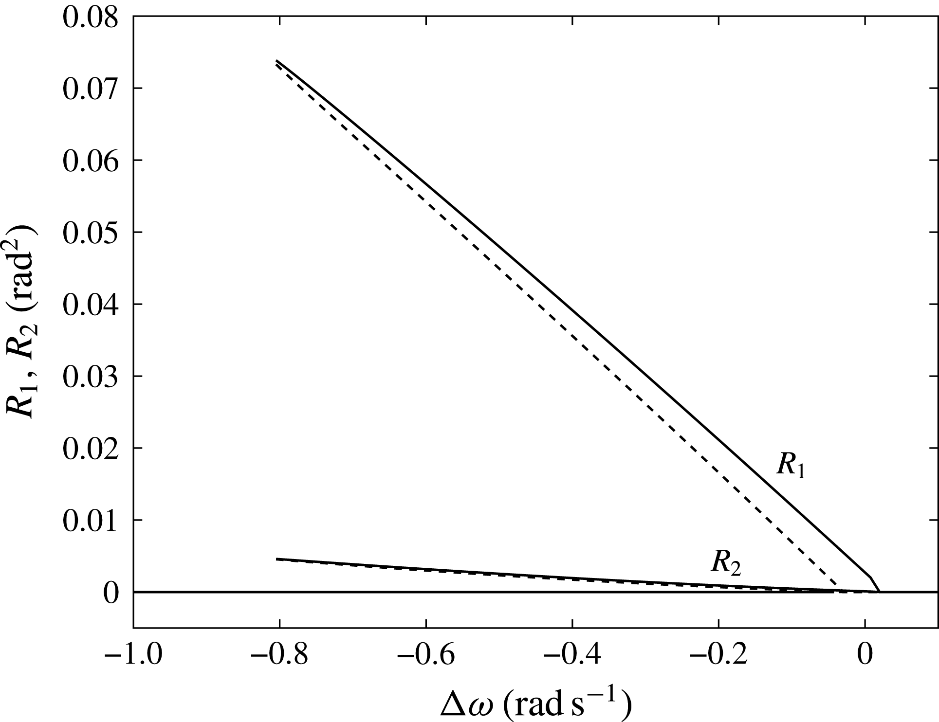
Figure 15. Equilibrium branches of
 $R_{1}$
ad
$R_{1}$
ad
 $R_{2}$
versus detuning of the incident wave
$R_{2}$
versus detuning of the incident wave
 $\unicode[STIX]{x0394}\unicode[STIX]{x1D714}$
. The solid lines represent the stable equilibrium branch while the dotted lines represent the unstable branch.
$\unicode[STIX]{x0394}\unicode[STIX]{x1D714}$
. The solid lines represent the stable equilibrium branch while the dotted lines represent the unstable branch.
At this point, we evaluate the efficiency of the system excited through mode-mode interactions. Figure 16 shows the behaviour of
 ${\mathcal{C}}^{F}$
versus the frequency of the incident waves. The maximum of the capture factor is
${\mathcal{C}}^{F}$
versus the frequency of the incident waves. The maximum of the capture factor is
 ${\sim}0.25$
, hence the effect of triad interaction is not as significant as the subharmonic case (see figure 6) but positive anyway.
${\sim}0.25$
, hence the effect of triad interaction is not as significant as the subharmonic case (see figure 6) but positive anyway.
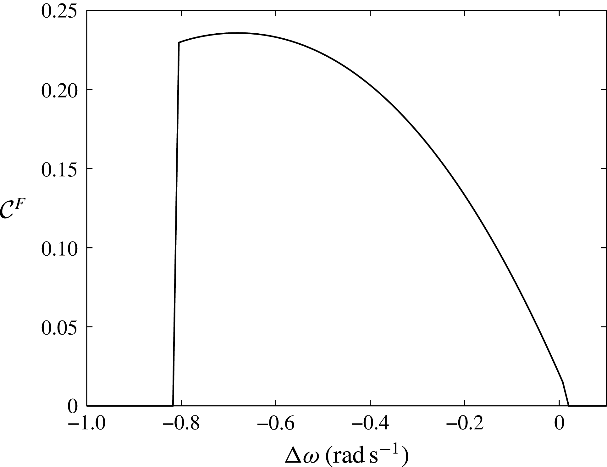
Figure 16. Behaviour of the capture factor due to triad resonance. Mode–mode interaction yields smaller values of
 ${\mathcal{C}}^{F}$
than the subharmonic resonance of a single mode.
${\mathcal{C}}^{F}$
than the subharmonic resonance of a single mode.
6 Conclusions
We have investigated theoretically the nonlinear effects on the performance of an array of oscillating wave surge converters in a channel. We extended the theory of Sammarco et al. (Reference Sammarco, Tran and Mei1997a
,Reference Sammarco, Tran, Gottlieb and Mei
b
) using scales which simplified considerably the required algebra for the coefficients of the Stuart–Landau evolution equation. This is because unlike the Venice gates, the OWSCs considered here do not span the entire water depth but are placed upon a vertical fixed wall on a rigid bottom. The dependence of the coefficients on the eigenfrequency of the system has been examined. We have derived a formula to evaluate the maximum capture factor in uniform incident waves and found that subharmonic excitation yields very large values of the capture factor. Moreover we showed that the array with large eigenfrequency induces an increase in the efficiency, hence heavier gates should be avoided in order to maximize energy production in nonlinear regimes. The dependence of the evolution equation coefficients on the eigenfrequency of the system has allowed us to determine thresholds of instability, equilibrium points of the dynamical system and the optimal values of the PTO coefficients which maximize power output. We have shown that gates with large buoyancy yield the array susceptible to subharmonic resonance, conversely, heavier gates are difficult to resonate. Detailed analysis was performed to see the effects of modulated incident waves on the dynamics of the array. We found thresholds above which homoclinic tangles and so chaotic regimes occur. We have shown that arrays with large eigenfrequency can exhibit chaos for a broader range of long-wave forcing frequencies. Numerical investigation of the non-autonomous dynamical system has allowed us to find bifurcation scenarios. By increasing the amplitude of the incident wave envelope we have reproduced period doubling cascades, chaotic bands and periodic windows. We have found that chaos disappears for large values of the periodic modulation. The response of the array is then subharmonic with the gate envelope and a frequency downshift of the peak power spectrum occurs. The efficiency of the system decreases significantly when period doubling and chaotic regimes occur. Finally we analysed the case of mode–mode interactions. We have found that effects of triad interactions on the generated power are not as significant than the pure subharmonic case, yet relevant. However this final investigation could be important for a fuller understanding of OWSCs complicated dynamics and to facilitate interpretation of experimental data results. We have assumed that the torque exerted by the ideal PTO increases linearly with the angular velocity of the gate. We have obtained that nonlinear resonance is possible for PTO coefficient values at
 $O(\unicode[STIX]{x1D716}^{2})$
. Several mechanisms not considered here such as friction losses, viscous damping and nonlinear PTO laws clearly influence the gate dynamics. However, to analyse these higher-order effects it is necessary also to study in detail the mechanics of a specific generator. This subject will be investigated soon. A second theoretical question remains, i.e. the analysis of the subharmonic resonance in open sea where natural modes of a finite array of OWSCs are nearly trapped and radiate energy. These questions represent a fairly open and challenging research subject and will be addressed in the near future to better understand the dynamics of such devices.
$O(\unicode[STIX]{x1D716}^{2})$
. Several mechanisms not considered here such as friction losses, viscous damping and nonlinear PTO laws clearly influence the gate dynamics. However, to analyse these higher-order effects it is necessary also to study in detail the mechanics of a specific generator. This subject will be investigated soon. A second theoretical question remains, i.e. the analysis of the subharmonic resonance in open sea where natural modes of a finite array of OWSCs are nearly trapped and radiate energy. These questions represent a fairly open and challenging research subject and will be addressed in the near future to better understand the dynamics of such devices.
Acknowledgements
This research was partially funded by ‘Sales SpA’. The authors would like to mention that without Professor C. C. Mei’s virtual supervision, none of this research would have been possible. Fruitful discussions with Dr E. Renzi are kindly acknowledged.
Appendix A. Details of the coefficient
$\unicode[STIX]{x1D6E5}_{pln}$

Following the same steps for the second-order solution of § 4.2 we obtain
 $$\begin{eqnarray}\displaystyle \unicode[STIX]{x1D6E5}_{pl1} & = & \displaystyle \frac{1}{2\unicode[STIX]{x1D6FF}_{p}C_{l1}}\mathop{\sum }_{q=1}^{Q}\mathop{\sum }_{m=1}^{\infty }\mathop{\sum }_{n=0}^{\infty }\left\{\frac{\unicode[STIX]{x1D714}_{1}b_{(m+p)q1}b_{mq1}D_{n1}C_{ln11}}{C_{n1}}\left(\frac{1}{\unicode[STIX]{x1D6FC}_{mn1}}+\frac{1}{\unicode[STIX]{x1D6FC}_{(m+p)n1}}\right)\right.\nonumber\\ \displaystyle & & \displaystyle \left.-\,d\unicode[STIX]{x1D714}_{1}E_{l1}b_{(m+p)q1}b_{mq1}\right\},\end{eqnarray}$$
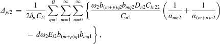 $$\begin{eqnarray}\displaystyle \unicode[STIX]{x1D6E5}_{pl2} & = & \displaystyle \frac{1}{2\unicode[STIX]{x1D6FF}_{p}C_{l2}}\mathop{\sum }_{q=1}^{Q}\mathop{\sum }_{m=1}^{\infty }\mathop{\sum }_{n=0}^{\infty }\left\{\frac{\unicode[STIX]{x1D714}_{2}b_{(m+p)q2}b_{mq2}D_{n2}C_{ln22}}{C_{n2}}\left(\frac{1}{\unicode[STIX]{x1D6FC}_{mn2}}+\frac{1}{\unicode[STIX]{x1D6FC}_{(m+p)n2}}\right)\right.\nonumber\\ \displaystyle & & \displaystyle \left.-\,d\unicode[STIX]{x1D714}_{2}E_{l2}b_{(m+p)q1}b_{mq1}\right\},\end{eqnarray}$$
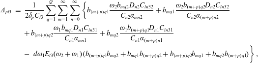 $$\begin{eqnarray}\displaystyle \unicode[STIX]{x1D6E5}_{pl3} & = & \displaystyle \frac{1}{2\unicode[STIX]{x1D6FF}_{p}C_{l3}}\mathop{\sum }_{q=1}^{Q}\mathop{\sum }_{m=1}^{\infty }\mathop{\sum }_{n=0}^{\infty }\left\{b_{(m+p)q1}\frac{\unicode[STIX]{x1D714}_{2}b_{mq2}D_{n2}C_{ln32}}{C_{n2}\unicode[STIX]{x1D6FC}_{mn2}}+b_{mq1}\frac{\unicode[STIX]{x1D714}_{2}b_{(m+p)q2}D_{n2}C_{ln32}}{C_{n2}\unicode[STIX]{x1D6FC}_{(m+p)n2}}\right.\nonumber\\ \displaystyle & & \displaystyle +\,b_{(m+p)q2}\frac{\unicode[STIX]{x1D714}_{1}b_{mq1}D_{n1}C_{ln31}}{C_{n1}\unicode[STIX]{x1D6FC}_{mn1}}+b_{mq2}\frac{\unicode[STIX]{x1D714}_{1}b_{(m+p)q1}D_{n1}C_{ln31}}{C_{n1}\unicode[STIX]{x1D6FC}_{(m+p)n1}}\nonumber\\ \displaystyle & & \displaystyle -\left.\,d\unicode[STIX]{x1D714}_{1}E_{l3}(\unicode[STIX]{x1D714}_{2}+\unicode[STIX]{x1D714}_{1})(b_{(m+p)q1}b_{mq2}+b_{mq1}b_{(m+p)q2}+b_{(m+p)q2}b_{mq1}+b_{mq2}b_{(m+p)q1})\right\},\nonumber\\ \displaystyle & & \displaystyle\end{eqnarray}$$
 $$\begin{eqnarray}\displaystyle \unicode[STIX]{x1D6E5}_{pl4} & = & \displaystyle \frac{1}{2\unicode[STIX]{x1D6FF}_{p}C_{l4}}\mathop{\sum }_{q=1}^{Q}\mathop{\sum }_{m=1}^{\infty }\mathop{\sum }_{n=0}^{\infty }\left\{b_{(m+p)q1}\frac{\unicode[STIX]{x1D714}_{2}b_{mq2}D_{n2}C_{ln42}}{C_{n2}\unicode[STIX]{x1D6FC}_{mn2}}+b_{mq1}\frac{\unicode[STIX]{x1D714}_{2}b_{(m+p)q2}D_{n2}C_{ln42}}{C_{n2}\unicode[STIX]{x1D6FC}_{(m+p)n2}}\right.\nonumber\\ \displaystyle & & \displaystyle -\,b_{(m+p)q2}\frac{\unicode[STIX]{x1D714}_{1}b_{mq1}D_{n1}C_{ln41}}{C_{n1}\unicode[STIX]{x1D6FC}_{mn1}}-b_{mq2}\frac{\unicode[STIX]{x1D714}_{1}b_{(m+p)q1}D_{n1}C_{ln41}}{C_{n1}\unicode[STIX]{x1D6FC}_{(m+p)n1}}\nonumber\\ \displaystyle & & \displaystyle -\left.\,d\unicode[STIX]{x1D714}_{1}E_{l4}(\unicode[STIX]{x1D714}_{2}-\unicode[STIX]{x1D714}_{1})(b_{(m+p)q1}b_{mq2}+b_{mq1}b_{(m+p)q2}+b_{(m+p)q2}b_{mq1}+b_{mq2}b_{(m+p)q1})\right\},\nonumber\\ \displaystyle & & \displaystyle\end{eqnarray}$$
where the coefficients
 $C_{ln1}$
and
$C_{ln1}$
and
 $C_{ln2}$
have the same form as (4.33), while
$C_{ln2}$
have the same form as (4.33), while
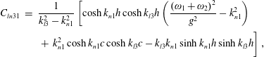 $$\begin{eqnarray}\displaystyle C_{ln31} & = & \displaystyle \frac{1}{k_{l3}^{2}-k_{n1}^{2}}\left[\cosh k_{n1}h\cosh k_{l3}h\left(\frac{\left(\unicode[STIX]{x1D714}_{1}+\unicode[STIX]{x1D714}_{2}\right)^{2}}{g^{2}}-k_{n1}^{2}\right)\right.\nonumber\\ \displaystyle & & \displaystyle \left.+\,k_{n1}^{2}\cosh k_{n1}c\cosh k_{l3}c-k_{l3}k_{n1}\sinh k_{n1}h\sinh k_{l3}h\right],\end{eqnarray}$$
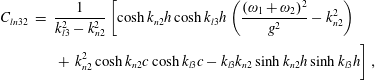 $$\begin{eqnarray}\displaystyle C_{ln32} & = & \displaystyle \frac{1}{k_{l3}^{2}-k_{n2}^{2}}\left[\cosh k_{n2}h\cosh k_{l3}h\left(\frac{(\unicode[STIX]{x1D714}_{1}+\unicode[STIX]{x1D714}_{2})^{2}}{g^{2}}-k_{n2}^{2}\right)\right.\nonumber\\ \displaystyle & & \displaystyle \left.+\,k_{n2}^{2}\cosh k_{n2}c\cosh k_{l3}c-k_{l3}k_{n2}\sinh k_{n2}h\sinh k_{l3}h\right],\end{eqnarray}$$
 $$\begin{eqnarray}\displaystyle C_{ln41} & = & \displaystyle \frac{1}{k_{l4}^{2}-k_{n1}^{2}}\left[\cosh k_{n1}h\cosh k_{l4}h\left(\frac{(\unicode[STIX]{x1D714}_{2}-\unicode[STIX]{x1D714}_{1})^{2}}{g^{2}}-k_{n1}^{2}\right)\right.\nonumber\\ \displaystyle & & \displaystyle \left.+\,k_{n1}^{2}\cosh k_{n1}c\cosh k_{l3}c-k_{l4}k_{n1}\sinh k_{n1}h\sinh k_{l4}h\right],\end{eqnarray}$$
 $$\begin{eqnarray}\displaystyle C_{ln42} & = & \displaystyle \frac{1}{k_{l4}^{2}-k_{n2}^{2}}\left[\cosh k_{n2}h\cosh k_{l4}h\left(\frac{\left(\unicode[STIX]{x1D714}_{2}-\unicode[STIX]{x1D714}_{1}\right)^{2}}{g^{2}}-k_{n2}^{2}\right)\right.\nonumber\\ \displaystyle & & \displaystyle \left.+\,k_{n2}^{2}\cosh k_{n2}c\cosh k_{l4}c-k_{l4}k_{n2}\sinh k_{n2}h\sinh k_{l4}h\right],\end{eqnarray}$$
 $$\begin{eqnarray}\displaystyle E_{lj} & = & \displaystyle \frac{1}{k_{lj}}(\sinh k_{lj}h-\sinh k_{lj}c),\quad j=1,\ldots ,4.\end{eqnarray}$$
Appendix B. Details of the forcing terms for the solvability condition (5.21)
Recall the solvability condition for each
 $j$
th harmonic:
$j$
th harmonic:
 $$\begin{eqnarray}\displaystyle & & \displaystyle \frac{\unicode[STIX]{x1D714}_{j}^{2}}{g}\int _{0}^{b}\,\text{d}y\left(\int _{-\infty }^{0}f_{1j}^{-}{\mathcal{F}}_{3j}^{-}\,\text{d}x-\int _{0}^{\infty }f_{1j}^{+}{\mathcal{F}}_{3j}^{+}\,\text{d}x\right)\nonumber\\ \displaystyle & & \displaystyle \quad +\,2\int _{0}^{b}\,\text{d}y\int _{-h}^{0}\overline{f_{j}{\mathcal{G}}_{3j}}\,\text{d}z+\mathop{\sum }_{q=1}^{Q}\left(\frac{\text{i}{\mathcal{D}}_{3j}r_{1jq}}{\unicode[STIX]{x1D70C}}-\frac{\unicode[STIX]{x1D708}_{pto}r_{1jq}^{2}\unicode[STIX]{x1D714}_{j}\unicode[STIX]{x1D703}_{j}}{\unicode[STIX]{x1D70C}\unicode[STIX]{x1D716}^{2}}\right)=0,\quad j=1,2.\end{eqnarray}$$
The forcing term for the free-surface mixed condition is defined as
 $$\begin{eqnarray}{\mathcal{F}}_{3j}^{\pm }=\pm \frac{2f_{1j}^{\pm }\unicode[STIX]{x1D703}_{t_{j}}}{\unicode[STIX]{x1D714}_{j}},\quad j=1,2,\end{eqnarray}$$
the forcing terms for the kinematic condition on the gates are respectively
 $$\begin{eqnarray}\displaystyle {\mathcal{G}}_{31}^{\pm } & = & \displaystyle -\{[\unicode[STIX]{x1D703}_{11}|\unicode[STIX]{x1D703}_{12}|^{2}(\text{i}r_{12q}\,f_{23_{z}}^{\pm }-\text{i}r_{12q}\,f_{24_{z}}^{\pm ^{\ast }})+\unicode[STIX]{x1D703}_{11}|\unicode[STIX]{x1D703}_{11}|^{2}\text{i}\,f_{11_{z}}r_{11q}]\nonumber\\ \displaystyle & & \displaystyle -\,A\unicode[STIX]{x1D703}_{12}^{\ast }(\unicode[STIX]{x1D719}_{z}^{\pm A}r_{12q})-r_{11q}\unicode[STIX]{x1D703}_{11_{t}}(z+h_{p})\pm 2\unicode[STIX]{x1D703}_{11}|\unicode[STIX]{x1D703}_{11}|^{2}\,d\unicode[STIX]{x1D714}_{1}\,f_{21}r_{11p}\nonumber\\ \displaystyle & & \displaystyle \pm \,\unicode[STIX]{x1D703}_{11}|\unicode[STIX]{x1D703}_{12}|^{2}\,d(\unicode[STIX]{x1D714}_{1}+\unicode[STIX]{x1D714}_{2})f_{23}r_{12q}\nonumber\\ \displaystyle & & \displaystyle \pm \,\unicode[STIX]{x1D703}_{11}|\unicode[STIX]{x1D703}_{12}|^{2}\,d(\unicode[STIX]{x1D714}_{2}-\unicode[STIX]{x1D714}_{1})f_{24}^{\ast }r_{12q}\!\}H(z+h-c),\end{eqnarray}$$
and
 $$\begin{eqnarray}\displaystyle {\mathcal{G}}_{32}^{\pm } & = & \displaystyle -\{[\unicode[STIX]{x1D703}_{12}|\unicode[STIX]{x1D703}_{11}|^{2}(\text{i}r_{11q}\,f_{23_{z}}^{\pm }+\text{i}r_{11q}\,f_{24_{z}}^{\pm })+\unicode[STIX]{x1D703}_{12}|\unicode[STIX]{x1D703}_{12}|^{2}\text{i}\,f_{12_{z}}r_{12q}]\nonumber\\ \displaystyle & & \displaystyle -\,A\unicode[STIX]{x1D703}_{11}^{\ast }(\unicode[STIX]{x1D719}_{z}^{\pm A}r_{11q})-r_{12q}\unicode[STIX]{x1D703}_{12_{t}}(z+h_{p})\pm 2\unicode[STIX]{x1D703}_{12}|\unicode[STIX]{x1D703}_{12}|^{2}\,d\unicode[STIX]{x1D714}_{2}\,f_{22}r_{12p}\nonumber\\ \displaystyle & & \displaystyle \pm \,\unicode[STIX]{x1D703}_{12}|\unicode[STIX]{x1D703}_{11}|^{2}\,d(\unicode[STIX]{x1D714}_{1}+\unicode[STIX]{x1D714}_{2})f_{23}r_{11p}\nonumber\\ \displaystyle & & \displaystyle \pm \,\unicode[STIX]{x1D703}_{12}|\unicode[STIX]{x1D703}_{11}|^{2}\,d(\unicode[STIX]{x1D714}_{2}-\unicode[STIX]{x1D714}_{1})f_{24}r_{11p}\!\}H(z+h-c),\end{eqnarray}$$
while the remaining forcing terms for the equation of motion of both modal oscillations are given by
 $$\begin{eqnarray}\displaystyle {\mathcal{D}}_{31}^{\pm } & = & \displaystyle -\unicode[STIX]{x1D70C}\int _{(q-1)a}^{qa}\,\text{d}y\left\{\int _{-h_{p}}^{0}\,\text{d}z[\!-6f_{11}r_{11q}^{2}\unicode[STIX]{x1D703}_{11}|\unicode[STIX]{x1D703}_{11}|^{2}\unicode[STIX]{x1D714}_{1}-6f_{12}r_{12q}r_{11q}\unicode[STIX]{x1D703}_{11}|\unicode[STIX]{x1D703}_{12}|^{2}\unicode[STIX]{x1D714}_{2}\right.\nonumber\\ \displaystyle & & \displaystyle -\,4f_{11}r_{12q}^{2}\unicode[STIX]{x1D703}_{11}|\unicode[STIX]{x1D703}_{12}|^{2}\unicode[STIX]{x1D714}_{1}-2\text{i}f_{11}\unicode[STIX]{x1D703}_{11_{t}}\! ](z+h_{p})+\frac{f_{11}^{3}\unicode[STIX]{x1D714}_{1}^{3}}{g^{2}}\unicode[STIX]{x1D703}_{11}|\unicode[STIX]{x1D703}_{11}|^{2}+\frac{f_{12}^{2}\,f_{11}\unicode[STIX]{x1D714}_{1}\unicode[STIX]{x1D714}_{2}^{2}}{g^{2}}\unicode[STIX]{x1D703}_{11}|\unicode[STIX]{x1D703}_{12}|^{2}\nonumber\\ \displaystyle & & \displaystyle +\,2h_{p}\unicode[STIX]{x1D6E5}\left[\frac{f_{12}\unicode[STIX]{x1D714}_{2}}{g}f_{24}^{\ast }(\unicode[STIX]{x1D714}_{2}-\unicode[STIX]{x1D714}_{1})\unicode[STIX]{x1D703}_{11}|\unicode[STIX]{x1D703}_{12}|^{2}+\frac{f_{12}\unicode[STIX]{x1D714}_{2}}{g}f_{23}(\unicode[STIX]{x1D714}_{2}+\unicode[STIX]{x1D714}_{1})\unicode[STIX]{x1D703}_{11}|\unicode[STIX]{x1D703}_{12}|^{2}\right.\nonumber\\ \displaystyle & & \displaystyle +\left.\left.\,2\frac{f_{11}\unicode[STIX]{x1D714}_{1}}{g}f_{21}\unicode[STIX]{x1D714}_{1}\unicode[STIX]{x1D703}_{11}|\unicode[STIX]{x1D703}_{11}|^{2}\right]-Ah_{p}(\unicode[STIX]{x1D714}_{1}+\unicode[STIX]{x1D714}_{2})\unicode[STIX]{x1D6E5}\left(\pm \frac{f_{12}\unicode[STIX]{x1D714}_{2}}{g}\unicode[STIX]{x1D719}^{\pm A}\unicode[STIX]{x1D703}_{12}^{\ast }\right)\right\}+2\unicode[STIX]{x1D714}_{1}Ir_{11q}\text{i}\unicode[STIX]{x1D703}_{11_{t}}\nonumber\\ \displaystyle & & \displaystyle +\,2\unicode[STIX]{x1D70C}\,d\int _{(q-1)a}^{qa}\,\text{d}y\int _{-h_{p}}^{0}\,\text{d}z(\!\unicode[STIX]{x1D703}_{11}|\unicode[STIX]{x1D703}_{11}|^{2}2\unicode[STIX]{x1D714}_{1}f_{21}r_{11q}+\unicode[STIX]{x1D703}_{11}|\unicode[STIX]{x1D703}_{12}|^{2}(\unicode[STIX]{x1D714}_{1}+\unicode[STIX]{x1D714}_{2})f_{23}r_{12q}\nonumber\\ \displaystyle & & \displaystyle +\,\unicode[STIX]{x1D703}_{11}|\unicode[STIX]{x1D703}_{12}|^{2}(\unicode[STIX]{x1D714}_{2}-\unicode[STIX]{x1D714}_{1})f_{24}^{\ast }r_{12q}\! )+\unicode[STIX]{x1D70C}\,d\int _{(q-1)a}^{qa}\,\text{d}y\left[\unicode[STIX]{x1D703}_{11}|\unicode[STIX]{x1D703}_{11}|^{2}3\frac{f_{11}^{2}\unicode[STIX]{x1D714}_{1}^{2}}{g}r_{11q}\right.\nonumber\\ \displaystyle & & \displaystyle \left.+\,\unicode[STIX]{x1D703}_{11}|\unicode[STIX]{x1D703}_{12}|^{2}\left(2\frac{f_{12}^{2}\unicode[STIX]{x1D714}_{2}^{2}}{g}r_{11q}+4\frac{f_{12}\unicode[STIX]{x1D714}_{2}f_{11}\unicode[STIX]{x1D714}_{1}}{g}r_{12q}\right)\right],\end{eqnarray}$$
and
 $$\begin{eqnarray}\displaystyle {\mathcal{D}}_{32}^{\pm } & = & \displaystyle -\unicode[STIX]{x1D70C}\int _{(q-1)a}^{qa}\,\text{d}y\left\{\int _{-h_{p}}^{0}\,\text{d}z[\!-6f_{12}r_{12q}^{2}\unicode[STIX]{x1D703}_{12}|\unicode[STIX]{x1D703}_{12}|^{2}\unicode[STIX]{x1D714}_{2}-6f_{11}r_{11q}\unicode[STIX]{x1D703}_{12q}\unicode[STIX]{x1D703}_{12}|\unicode[STIX]{x1D703}_{11}|^{2}\unicode[STIX]{x1D714}_{1}\right.\nonumber\\ \displaystyle & & \displaystyle -\,4f_{12}r_{11q}^{2}\unicode[STIX]{x1D703}_{12}|\unicode[STIX]{x1D703}_{11}|^{2}\unicode[STIX]{x1D714}_{1}-2\text{i}f_{12}\unicode[STIX]{x1D703}_{12_{t}}\! ](z+h_{p})+\frac{f_{12}^{3}\unicode[STIX]{x1D714}_{2}^{3}}{g^{2}}\unicode[STIX]{x1D703}_{12}|\unicode[STIX]{x1D703}_{12}|^{2}+\frac{f_{11}^{2}\unicode[STIX]{x1D714}_{1}^{2}f_{12}\unicode[STIX]{x1D714}_{2}}{g^{2}}\unicode[STIX]{x1D703}_{12}|\unicode[STIX]{x1D703}_{11}|^{2}\nonumber\\ \displaystyle & & \displaystyle +\,2h_{p}\unicode[STIX]{x1D6E5}\left[\frac{f_{11}\unicode[STIX]{x1D714}_{1}}{g}f_{24}(\unicode[STIX]{x1D714}_{2}-\unicode[STIX]{x1D714}_{1})\unicode[STIX]{x1D703}_{12}|\unicode[STIX]{x1D703}_{11}|^{2}+\frac{f_{11}\unicode[STIX]{x1D714}_{1}}{g}f_{23}(\unicode[STIX]{x1D714}_{2}+\unicode[STIX]{x1D714}_{1})\unicode[STIX]{x1D703}_{12}|\unicode[STIX]{x1D703}_{11}|^{2}\right.\nonumber\\ \displaystyle & & \displaystyle \left.\left.+\,2\frac{f_{12}\unicode[STIX]{x1D714}_{2}}{g}f_{22}\unicode[STIX]{x1D714}_{2}\unicode[STIX]{x1D703}_{12}|\unicode[STIX]{x1D703}_{12}|^{2}\right]-Ah_{p}(\unicode[STIX]{x1D714}_{1}+\unicode[STIX]{x1D714}_{2})\unicode[STIX]{x1D6E5}\left(\pm \frac{f_{11}\unicode[STIX]{x1D714}_{1}}{g}\unicode[STIX]{x1D719}^{\pm A}\unicode[STIX]{x1D703}_{11}^{\ast }\right)\right\}+2\unicode[STIX]{x1D714}_{1}Ir_{12q}\text{i}\unicode[STIX]{x1D703}_{12_{t}}\nonumber\\ \displaystyle & & \displaystyle +\,2\unicode[STIX]{x1D70C}d\int _{(q-1)a}^{qa}\,\text{d}y\int _{-h_{p}}^{0}\,\text{d}z(\!\unicode[STIX]{x1D703}_{12}|\unicode[STIX]{x1D703}_{12}|^{2}2\unicode[STIX]{x1D714}_{2}f_{22}r_{12q}+\unicode[STIX]{x1D703}_{12}|\unicode[STIX]{x1D703}_{11}|^{2}(\unicode[STIX]{x1D714}_{1}+\unicode[STIX]{x1D714}_{2})f_{23}r_{11q}\nonumber\\ \displaystyle & & \displaystyle +\,\unicode[STIX]{x1D703}_{12}|\unicode[STIX]{x1D703}_{11}|^{2}(\unicode[STIX]{x1D714}_{2}-\unicode[STIX]{x1D714}_{1})f_{24}r_{11q}\! )+\unicode[STIX]{x1D70C}\,d\int _{(q-1)a}^{qa}\,\text{d}y\left[\unicode[STIX]{x1D703}_{12}|\unicode[STIX]{x1D703}_{12}|^{2}3\frac{f_{12}^{2}\unicode[STIX]{x1D714}_{2}^{2}}{g}r_{12q}\right.\nonumber\\ \displaystyle & & \displaystyle \left.+\,\unicode[STIX]{x1D703}_{12}|\unicode[STIX]{x1D703}_{11}|^{2}\left(2\frac{f_{11}^{2}\unicode[STIX]{x1D714}_{1}^{2}}{g}r_{12q}+4\frac{f_{11}\unicode[STIX]{x1D714}_{1}f_{12}\unicode[STIX]{x1D714}_{2}}{g}r_{11q}\right)\right].\end{eqnarray}$$


