Balancing the Fluorescence Imaging Budget for All-Optical Neurophysiology Experiments

Abstract

The goal of this chapter is to establish a framework to evaluate imaging methodologies for all-optical neurophysiology experiments. This is not an exhaustive review of fluorescent indicators and imaging modalities but rather aims to distill the functional imaging principles driving the choice of both. Scientific priorities determine whether the imaging strategy is based on an “optimal fluorescent indicator” or “optimal imaging modality.” The choice of the first constrains the choice of the second due to each’s contributions to the fluorescence budget and signal-to-noise ratio of time-varying fluorescence changes.

1 Introduction

Optical methods provide powerful means to investigate the structure and function of many neurons simultaneously. Importantly, photons can be focused to, and imaged from, multiple neurons in parallel to control and detect their activity. Several new imaging strategies are developed every year, and neurophysiologists must navigate growing stacks of methods papers, microscope, and laser adverts to identify which modality can best achieve the scientific goals of their experiments. There are a broad set of competing requirements on the techniques used to image neuronal activity including speed, depth, spectral separation, robustness to scattering, and motion artifacts. The goal of this chapter is to distill the trade-offs driving choice of imaging strategy for all-optical experiments.

We begin by detailing two key challenges to imaging neuronal activity in intact brains. We then define signal-to-noise ratio and the concept of a “fluorescence budget,” which ultimately determines how small and fast of a transient signal can be resolved by a given imaging configuration. We then detail how the choice of fluorophore, in particular indicators of calcium and membrane potential, and imaging modality relate to the fluorescence budget, and the trade-offs inherent to the choice of each.

2 Key Challenges to Imaging Neuronal Activity

2.1 Challenge 1: Brains Are Three-Dimensional

Brains are three-dimensional (3D), while conventional microscopes image one plane at a time. A widefield fluorescence microscope (Fig. 1, left) excites fluorescence throughout a 3D volume and images fluorescence from a single plane. Unless the fluorophore itself is restricted to one plane (e.g., culture cell monolayers), fluorescence is excited outside of the plane of focus (Fig. 2, left). At the camera chip, this out-of-focus light reduces the contrast of the in-focus image. Worse, in the context of imaging calcium or voltage signals, the labeled out-of-focus cells have individually varying fluorescence time courses that contribute to the in-focus time course. This makes standard widefield fluorescence imaging with single-cell resolution often untenable in densely labeled 3D samples. Many techniques have been developed to restrict fluorescence excitation (two/three-photon, light-sheet microscopy) and/or collection (confocal variants) to a single plane of focus and/or remove out-of-focus fluorescence in post-processing by combining multiple images with structured illumination [22, 63, 73, 76]. The ability to localize fluorescence to a plane orthogonal to the optical axis is termed “optical sectioning.” This “optical section” can scan orthogonal to the plane of focus to build up a volumetric image plane by plane.

Fig. 1

Widefield, one-photon imaging (left) and multiphoton scanning (right) imaging modalities; not to scale

Fig. 2

The challenges of 3D imaging in brain tissue. (a) Techniques that are not optically sectioning suffer from blur caused by the collection of light from out-of-focus planes. (b) Light rays can be scattered before exiting the tissue, changing their apparent origin. In aggregate, this leads to a blurring effect that drastically increases with depth. Reproduced from [88], CC BY-SA 4.0

2.2 Challenge 2: (Most) Brains Scatter Light

While certain model organisms (e.g., larval zebrafish, C. elegans) are transparent, most brains, especially mammalian brains, scatter light strongly. Fluorescence excitation efficiency decreases with increasing imaging depth as excitation light is scattered and absorbed, resulting in the degradation of the excitation point-spread function (PSF). Moreover, light excited in one spatial location can be scattered before collection and detected as though arising from somewhere else (Fig. 2, right). This degrades image contrast and confuses analysis of fluorescence time courses in adjacent areas.

Together, out-of-focus fluorescence and scattered fluorescence produce blurring, which drastically increases with imaging depth [46]. The need for optical sectioning and robustness to scattering has driven development and application of two- [30] and three-photon [45, 121] (or “multiphoton”) point scanning modalities, which achieve both. Due to non-linear dependence on excitation intensity, two- and three-photon fluorescence excited by high numerical aperture (NA) focusing generates femtoliter fluorescence volumes. Non-descanned fluorescence generated at the focus, scattered and non-scattered, is collected through the objective onto a large area detector (Fig. 1, right), commonly a photomultiplier tube. Two-dimensional images or 3D volumes are built up point by point by scanning the focus. This strategy enables calcium-based imaging of action potentials (APs) at depths up to 1 mm in mouse brains [59]. These techniques optically section and are robust to scattering; for structural imaging in live brains, this is as close as we have to perfect. Why, therefore, consider a different strategy for functional imaging? The next section introduces the key concept and guiding principle to designing and selecting a modality to image neuronal activity: the “fluorescence budget.”

3 Signal-to-Noise Ratio Is King: Fluorescence Budget

The principal consideration guiding optical neurophysiology systems is the signal-to-noise ratio (SNR) of time-varying fluorescence changes. Here the term signal-to-noise ratio most commonly refers to the ratio of the amplitude of a time-varying signal (S) transient to the “baseline noise” (σ), typically the root mean square of the signal that precedes or follows a transient peak (Fig.3). Note that this definition differs from how signal-to-noise ratio is often defined in scientific and engineering disciplines (see Note 1). Note also that in this chapter we are dealing specifically with the SNR of temporal, not spatial, fluorescence changes.

Fig. 3

Signal-to-noise ratio can be defined as the ratio of the amplitude of a time-varying signal (S) transient to the “baseline noise” (σ)

The temporal SNR quantifies the ease with which a fluorescence transient can be resolved from a noisy time-varying signal. The SNR is equal to the product of the fractional change in fluorescence with respect to baseline, or “indicator sensitivity,” multiplied by the total fluorescence collected per location (pixel or voxel), per integration period, the “fluorescence budget” (see Note 2):

$$ SNR=\frac{\Delta F}{F_0}\sqrt{F_0}. $$

(1)

ΔF∕F₀ reflects the sensitivity of the indicator’s fluorescence to the physiological signal (e.g., membrane potential or calcium). The fluorescence budget, F₀, is given by

$$ {F}_0=\phi \kern2.22198pt {F}_{gen}, $$

(2)

where ϕ (unitless) is the fluorescence collection efficiency and F_gen (in photons) is the fluorescence generated per location (pixel or voxel), per integration period. ϕ is determined by an assortment of factors dependent on the sample, such as imaging depth, wavelength-specific absorption, scattering length, and anisotropy, and specific to the collection optics, such as acceptance angle (numerical aperture, NA) and detector efficiency [129]. ϕ quantifies what fraction of fluorescence is collected by the imaging system. The fluorescence generated is

$$ {F}_{gen}={R}_{Fl}\kern2.22198pt {C}_{Fl}\kern2.22198pt {V}_{Fl}\kern2.22198pt \Delta t, $$

(3)

where R_Fl is the fluorescence rate (photons/s/molecule), C_Fl is the fluorophore concentration (molecules/m³), V_Fl is the per location fluorescence excitation volume (m³), and Δt is the integration period (s). The fluorescence rate is given by

$$ {R}_{Fl}={\sigma}_n<{I}^n> $$

(4)

in photons/s where σ_n is the n-photon brightness (1-, 2-, or 3- photon), the wavelength-dependent product of cross-section and quantum yield (m²ⁿ sⁿ⁻¹/photonsⁿ⁻¹), and < Iⁿ >  is the time average of the fluorescence excitation intensity raised to the n-th power (photonsⁿ/m²ⁿ/sⁿ).¹ Ideally, < Iⁿ >  is maximized to increase SNR up to the limit of photobleaching, heating, and in the case of ultrafast pulsed excitation, non-linear damage thresholds. Substituting gives

$$ SNR=\frac{\Delta F}{F_0}\sqrt{\phi \kern2.22198pt {\sigma}_n<{I}^n>{C}_{Fl}\kern2.22198pt {V}_{Fl}\kern2.22198pt \Delta t}. $$

(5)

The two imaging modalities introduced in the previous section, widefield and multiphoton scanning, are at opposite extremes in terms of fluorescence budget. Widefield integrates photons from all locations in a two-dimensional frame simultaneously throughout the frame period, and hence:

$$ \Delta t=\frac{1}{R_{acq}{N}_Z}, $$

(6)

where R_acq is the frame acquisition rate and N_Z is the number of planes imaged per volume. In contrast, multiphoton point rastering modalities integrate fluorescence from each location for only a small fraction of the acquisition period

$$ \Delta t=\frac{1}{R_{acq}{N}_X{N}_Y{N}_Z}, $$

(7)

where N_X and N_Y are the lateral frame dimensions.

Consider the case where N_Z = 1 to image a single plane, such that R_acq is the frame rate, and compare the widefield to the multiphoton raster scan case. For the widefield case, Δt = 1∕R_acq. For the multiphoton scanning case, digitizing each frame for example as N_X = N_Y = 256 pixels, we see that Δt = 1∕(256²R_acq). If we base our SNR comparison solely on differences in Δt, we see that the SNR for the widefield case is $\sqrt{25{6}^2}=256$ times that of multiphoton scanning! Note that this factor could be even bigger if the scanning modality involves significant “dead time” (i.e., galvonometric scanner turn around). Cameras also require read-out time, during which they are not integrating photons; however, this is typically around 10 μs per line for a modern sCMOS camera, a small fraction of the frame period, while scanning dead time can be around 10–20% of each frame.

The optical sectioning and robustness to scattering achieved by 2P and 3P point scanning modalities over widefield comes at high cost to the fluorescence budget, F₀. Note that in the multiphoton point scanning case, F₀ is inversely proportional to the product of the number of locations (pixels or voxels, N_XN_YN_Z) monitored, and the rate at which they are monitored, R_acq. This implies that F₀ can be maintained by performing high R_acq acquisition of few locations or low R_acq acquisition of many locations. For example, at the high rate extreme, 10 kilohertz acquisition of voltage transients from a single “voxel” has been achieved in two photon by parking the beam over a dendritic spine [3]. At the other extreme, two-photon “mesoscopes” image FOVs multiple millimeters wide at low frame rates (0.1–10 Hz) [102, 106] using slow and highly sensitive calcium indicators [25, 29].

From Eq. 5, we see that SNR can be increased by: 1. use of a high sensitivity (large ΔF∕F₀) fluorescence reporter and/or 2. increasing F₀. F₀ can be increased by: maximizing ϕ with efficient photo-sensors, high collection NA, etc.; selecting a bright fluorophore and exciting it at wavelengths for which its brightness, σ_n, is highest; maximizing fluorophore concentration, C_Fl, and exciting and collecting fluorescence over the largest possible voxel, V_Fl; exciting the fluorophore with the highest feasible intensity, < Iⁿ > ; and maximizing integration time, Δt. Table 1 summarizes the parameters contributing to SNR of functional fluorescence signals. The next sections discuss trade-offs driving choice of fluorophore and imaging modality.

Table 1 Summary of variables determining temporal SNR for functional fluorescence imaging

4 Choosing a Fluorescent Indicator

A fluorescent indicator is an organic molecule or protein functionalized to transduce biophysical changes into changes in fluorescence. Most commonly used are indicators that respond to changes in membrane potential [11, 13] and calcium [7, 112], but others exist that respond to pH [93, 94], sodium [56, 61], and neurotransmitter concentration including glutamate [69, 70], acetylcholine [52], or GABA [71]. With regard to temporal SNR, the key parameters of such a molecule include its sensitivity (ΔF∕F₀) and brightness (σ_n) as described above and its temporal profile.

4.1 Temporal Considerations

Here, indicator “temporal profile” refers to the convolution of the time course of a biophysical process (e.g., fast membrane potential variations vs. slow changes in calcium or neurotransmitter concentration) with the kinetics of the fluorescent indicator. Here we refer to τ_Off as a general term for the rate of decay back to baseline of the fluorescence transient induced by an action potential or other brief event. We note, however, that many indicators’ kinetics are not described by a simple mono-exponential decay. Importantly, τ_Off determines the minimum R_acq (and hence maximum Δt) able to resolve the time-varying signal without aliasing. For example, some highly sensitive Förster resonance energy transfer (FRET)-based voltage indicators temporally low pass filter fast events such as action potentials due to slow translocation of mobile charges in the plasma membrane [41]. While considered a disadvantage in most scientific contexts, this low pass filtering is an advantage for imaging, as slower transient changes in fluorescence can be imaged at lower rates R_acq without aliasing, thereby increasing Δt and F₀. The minimum R_acq is defined by the functional fluorescence temporal profile and also by the goals of the experiment. For instance, R_acq can be relatively low for mere transient detection but must be much higher to characterize transient timing and kinetics [90]. The implications of differing τ_Off for imaging strategy design can be readily appreciated through comparison of calcium and membrane potential indicators for neuronal AP detection.

4.2 Membrane Potential vs. Calcium

The majority of all-optical neurophysiology experiments monitor neuronal membrane potential, either directly with voltage-sensitive fluorophores or indirectly through fluorophores sensitive to calcium concentration. In most cases, calcium transients are monitored to detect when a neuron fires an action potential; so why not always choose voltage-sensitive fluorophores to image membrane potential directly? The particular challenges of imaging membrane potential compared to calcium are summarized in Fig. 4. First, the physiological signal kinetics are fast, milliseconds in the case of action potentials, necessitating high R_acq. High sampling rates limit the available photon integration time, Δt, demanding brighter (high σ_n) indicators for adequate SNR as discussed in Note 2.

Fig. 4

The challenges of voltage imaging. Three issues make voltage imaging more challenging than calcium imaging. First, faster intrinsic kinetics limit the photon integration period. Second, voltage indicators must lie in the membrane or degrade the signal; this limits the volume of indicators that can be integrated to measure the signal. Lastly, membranes where signal arises are tightly packed in the brain; fluorescent signals from overlapping membranes wash out single-cell signals. Adapted from original in [88], CC BY-SA 4.0

While calcium indicators are distributed throughout the cytosolic volume, voltage indicators are confined to the membrane. The 100-mV membrane potential fluctuation during an action potential leads to an electric field change of around 3 × 10⁷ V/m across the 3-nm-thick plasma membrane. Despite this large field, the fluorescent indicator’s sensor molecules must orient across the neuron’s external plasma membrane to sense any changes. This causes multiple challenges. First, the potential for physiological disruption by membrane indicator expression limits labeling density (and hence C_Fl). Membrane capacitance also increases with the number of charged or polarizable molecules in the plasma membrane, and over-labeling can even abolish action potentials completely [18]. Second, highly lipophilic dyes or poorly targeted genetic constructs can label membranes non-specifically, including internal membranes not exposed to changing fields. This increases background relative to the voltage-dependent signal, effectively reducing ΔF∕F₀ and proportionally the SNR. Third, overlapping membranes from adjacent cellular processes in densely labeled samples are indistinguishable in most microscope images. This results in signal mixing, especially with widefield single-photon illumination. Voltage transients from individual cells are then “washed out” by the bright background from adjacent cells.

Calcium indicators are widely used in neuroscience to indirectly detect APs due to their relative ease of use compared to voltage indicators. These indicators change brightness when bound to Ca²⁺ ions. As AP firing in most neurons is accompanied by a rapid, transient increase in intracellular Ca²⁺ concentration, calcium sensors report a proxy for neuronal spiking. The increase in intracellular Ca²⁺ on AP firing due to the opening of voltage-gated channels can be “amplified” by release from internal stores [14] and results in up to an order of magnitude change with a slow decay over hundreds of milliseconds [14, 60]. This low pass filters AP waveforms and enables longer integration times (Δt) without signal aliasing, increasing photon counts. Many more calcium indicators can be loaded into the cell compared to voltage indicators as calcium concentration changes throughout the cytosolic volume, increasing signal brightness. Combined, these advantages have made calcium imaging a popular technique enabling high SNR optical recording of AP activity.

Despite these advantages, there remain significant drawbacks to calcium indicators that limit their applicability. Calcium transients are not exclusively linked to action potential firing in all neurons [42, 68, 74]. AP-evoked calcium dynamics are also slow compared to APs, and indicator kinetics often further reduce the fluorescence response speed. Although beneficial for imaging, this limits the accuracy with which the timing of the underlying electrophysiological activity can be estimated, even when the link between APs and calcium transients is clear. Further complications confusing the link between indicator brightness and electrophysiology include indicator saturation, intrinsic and indicator buffering, and diffusion biophysics [95]. Increased calcium buffering due to high indicator concentrations has also resulted in pathology [72, 105]. Possibly the most important disadvantage to calcium indicators is their inability to report subthreshold membrane potential changes. Calcium indicators can be used to image calcium influx related to synaptic events [17]; however, at the soma, they report suprathreshold AP activity. These factors have motivated development of better optical, chemical, and biological techniques for imaging voltage in neurons. Both the relatively low ΔF∕F₀ of these indicators and high required R_Fl, however, necessitate careful consideration of the photon budget (F₀) when developing imaging strategies.

In summary, voltage indicators feature small ΔF∕F₀ and fast kinetics (short τ_Off) that require imaging with high fluorescence budget, especially long Δt, modalities (e.g., widefield, light field) to maintain SNR. Calcium indicators feature comparatively high ΔF∕F₀ and calcium transients decay slowly, enabling imaging at low R_acq. These features render calcium indicators eminently compatible with low fluorescence budget modalities such as multiphoton raster scanning.

4.3 Spectral Considerations

Of particular concern for all-optical experiments is avoiding spectral crosstalk between photostimulation and fluorescence excitation light. Such crosstalk comes in two types: imaging and physiological. Imaging crosstalk occurs when photons meant to stimulate neurons spuriously excite the functional fluorescent indicator. Imaging crosstalk can be avoided altogether if the photostimulation wavelength does not efficiently excite the indicator (e.g. [40]). If not, fortunately, transient artefacts due to imaging crosstalk can be predicted or measured, and subtracted, even in real time in some configurations [35], and generally do not affect the scientific integrity of the data. Physiological crosstalk occurs when light intended to excite the functional indicator fluorophore is spuriously absorbed by the opsin, causing neuronal de- or hyperpolarization. In contrast with optical crosstalk, physiological crosstalk, even subthreshold, undermines the scientific validity of the data by compromising the membrane potential, and in some cases action potential rate and timing, of the imaged neurons. Indeed the photocurrents spuriously generated by the imaging light cannot be subtracted; they must be prevented to realize the scientific potential of all-optical neurophysiology.

There are two ways to prevent physiological crosstalk in all-optical experiments: spectral separation and spatial separation. Spectral separation refers to exciting the indicator fluorophore at wavelengths at which the opsin actuator cross-section is so small that no photocurrents can be measured by whole-cell patch clamp in the opsin-transfected cells. Importantly, this control must be measured at the intensities and durations needed for imaging the fluorescent indicator. For one-photon excitation, this has been achieved by pairing blue–green-absorbing opsins with red-shifted calcium dyes [104], voltage dyes [64, 114, 119], GEVIs [1, 34, 47], and GECIs [7, 124]. Alternatively, red-shifted opsins, such as C1V1 [125], ReaChR [65], or Chrimson [57], can be combined with green-emitting calcium indicators (see also Chapters 3 and 4), although these red-shifted opsins exhibit 20%–30% actuation efficiency under blue-light excitation [116] and are thus more susceptible to spectral crosstalk than pairings where the opsin is excited at shorter wavelengths than the indicator. Spatial separation refers to limiting [107] or eliminating the fluorescence excitation light incident on opsin-expressing cells and substructures. For instance in cases where the opsin is targeted to the soma [10, 67, 99] or to a specific neuronal subpopulation, the fluorescence excitation light could be patterned exclusively over non-opsin-expressing structures and cells. Efforts to reduce crosstalk in one-photon excitation schemes with large spectral overlap between opsin actuators and indicators (e.g., the actuator channelrhodopsin-2 [ChR2] + GCaMP calcium reporters) have minimized read-out light intensities (< I_n > ) [44, 107] to the detriment of SNR.

Multiphoton schemes for opsin actuation and imaging have yet to demonstrate a configuration completely free of physiological crosstalk. Finding a scheme in which the imaging laser does not evoke spurious photocurrents, producing sub- and/or suprathreshold membrane potential changes, is especially difficult due to broad opsin two-photon action spectra. Spurious suprathreshold activation has been reduced or avoided by using opsins and indicators with partially separated absorption spectra (e.g., C1V1 with GCaMP6s [83]; ChR2, GtACR2, or stCoChR with jRCaMP1a [36, 37]) and by limiting the imaging dwell time, although subthreshold actuation may still occur. Broad multiphoton spectra can provide an advantage for imaging-only configurations (without an opsin) by exciting multiple fluorophores simultaneously with a single wavelength (e.g., green-emitting OGB-1 or GCaMP with red-emitting SR101 [16, 75]). Excitation to a higher-energy electronic excited state has also enabled multi-fluorophore three-photon imaging with a single wavelength [48].

4.4 Fluorophore Spatial Distribution

Of critical importance to SNR is the fluorescent indicator spatial distribution, both within a cell and within a population of cells. The fluorescent indicator properties determine the maximum ΔF∕F₀, but this is effectively reduced in proportion to the amount of “useless” or “background” fluorescence in the cell and surrounding space. Background fluorescence reduces the SNR as the non-signal-containing photons are collected from the same ROI as signal-containing photons, reducing the fractional change in fluorescence. If the baseline fluorescence rate from signal-containing molecules is given by F₀, and the rate of background fluorescence is given by F_B, then the fractional change in fluorescence is reduced to

$$ \frac{\Delta F}{F_0+{F}_B}=\left(1-{f}_B\right)\frac{\Delta F}{F_0},\kern1em \textrm{where}\kern1em {f}_B=\frac{F_B}{F_0+{F}_B}, $$

(8)

the fraction of fluorescence contributed by the background. The SNR is then given by

$$ \textrm{SNR}=\left(1-{f}_B\right)\frac{\Delta F}{F_0}\sqrt{F_0+{F}_B}=\sqrt{1-{f}_B}\frac{\Delta F}{F_0}\sqrt{F_0}=\sqrt{1-{f}_B}{\textrm{SNR}}_0, $$

(9)

as ${F}_0+{F}_B=\frac{F_0}{1-{f}_B}$ [58].

Dense fluorophore labeling poses problems especially for voltage indicators due to their membrane localization. Voltage signals in densely labeled samples cannot be resolved without indicator somatic restriction to reduce fluorescence contributions from overlapping adjacent processes (e.g., [2, 4, 117]) or imaging at sub-micron resolution, which has yet to be demonstrated. This problem is mitigated in preparations where the labeled cells are non-adjacent or “sparse.” For example, single neuron, single-trial action potential GEVI imaging has been achieved by expressing the GEVI strongly and sparsely in a subpopulation of cortical layer 2/3 excitatory neurons [90] due to the high effective ΔF∕F₀.

In summary, the sensitivity, brightness, kinetics, and spatial distribution of a fluorescent indicator determine which imaging modalities can resolve the functional fluorescence transients. Bright, slow, and sensitive indicators can boost temporal SNR for low fluorescence budget imaging modalities. For example, if interested in membrane potential, but wanting to track the activity of many cells with scattering-robust two-photon imaging, one can compensate two photon’s low fluorescence budget with a slow, bright calcium indicator.

5 SNR and Imaging Modality

Fluorescence imaging systems are comprised of two subsystems: (1) the fluorescence excitation subsystem and (2) the fluorescence detection subsystem. Here we detail how the characteristics of each subsystem contributes to temporal SNR.

5.1 Fluorescence Excitation

Regarding SNR, the fluorescence excitation subsystem can be characterized in terms of light intensity, < Iⁿ > , and the per pixel, per integration period excited volume, V_Fl. Together with the fluorophore cross-section (σ_n), concentration (C_Fl), integration period (Δt), and spatial distribution, these parameters determine the maximum available fluorescence excitation budget (F_gen; Eqs. 3, 4). The illumination wavelength and fluorophore cross-sections determine whether the system favors one-photon, two-photon, or three-photon fluorescence excitation. Two- and three-photon excitation requires ultrafast pulsed lasers with megahertz² repetition frequencies to achieve R_Fl sufficient for imaging. One-photon fluorescence excitation rates, R_Fl, vary widely depending on indicator brightness (σ₁) and illumination intensity (< I > ) and generally exceed R_Fl for two- and three-photon modalities, which typically excite < 0.1 photons per laser pulse [101].

5.1.1 Fluorescence Excitation Volume, V_Fl

The fluorescence excitation rate critically depends on the degree to which the fluorescence excitation is parallelized. Widefield excitation, which excites fluorescence in all locations throughout a volume simultaneously, features the highest degree of parallelization, thus maximizing the fluorescence excitation budget. Focusing a laser beam to a diffraction-limited point and serially scanning that point correspond to lowest parallelization and excitation budget. In between widefield and scanned point excitation, the excitation light can be sculpted into many forms, including a large point (scanned-temporal focusing; S-TeFo, [87, 118]), multiple scanned (spinning disk confocal [108, 126], multifocal 2P [15, 55, 78, 89, 98, 120, 127]) or static (computer-generated holography, [23, 32, 85, 122]) points, a line (TeFo line scanning [28], SLAP [53], vTWINS [103], Bessel beams [19, 66]), whole planes [5, 20, 51, 54, 82, 96, 97, 128], and extended shapes patterned directly onto structures of interest [21, 39, 79, 109, 110]. It is important to note that not all fluorescence photons contribute useful signal. For example, a higher proportion of photons excited through two-photon point scanning contribute to image formation compared to widefield imaging, where photons excited outside the plane of focus are not imaged and can smear the temporal signals extracted from in-focus ROIs. It is also important to note that V_Fl introduced earlier in this chapter refers to the per location fluorescence volume, not the total spot, line, or sheet volume, and therefore depends on the spatial discretization performed by the collection subsystem.

5.1.2 Fluorescence Integration Time, Δt

The fluorescence excitation subsystem determines the relationship between R_acq and Δt. In particular, for excitation that does not move or change shape during the acquisition period, Δt = 1∕R_acq. Scanning generally reduces Δt in proportion to the number of locations scanned. Table 2 summarizes Δt for the different scanned excitation shapes. Bearing in mind that $SNR\propto \sqrt{\Delta t}$, we appreciate the power of parallelization to boost the fluorescence budget (F₀), enabling imaging of smaller and faster signals, and/or over larger fields of view. Fluorescence parallelization, however, reduces robustness to scattering, as discussed next.

Table 2 Δt for the different excitation volume shapes in scanning configurations

5.2 Fluorescence Detection

The fluorescence detection system determines how the fluorescence excitation budget is exploited to form images. Sensors for fluorescence detection fall into two categories: single and multi-channel.

5.2.1 Single-Channel Detectors

Single-channel detectors, including photodiodes and photomultiplier tubes (PMTs), read out fluorescence intensity (or photons) as a function of time. Imaging is achieved by combining single-channel detectors with scanned fluorescence excitation through the process of “temporal multiplexing”: the localization of fluorescence based on when it was detected. Moreover, temporal multiplexing can be used to scan multiple areas or z-planes by alternating the focus of time sequential laser pulses [12, 24, 26, 49, 106, 118]). The degree of temporal multiplexing, along with the total rate of fluorescence excited from the sample (R_Fl), is ultimately determined by the indicator’s fluorescence lifetime [26].

Single-channel detection of point-scanned two- and three-photon fluorescence excitation features the highest achievable robustness to scattering and finest optical sectioning, owing to temporal multiplexing. These advantages, as previously discussed, are achieved at the cost of fluorescence excitation bandwidth, even when fluorescence rates (R_Fl) are maximized through pulse energies and repetition rates increased to the maximum allowable by photo-damage thresholds and fluorophore lifetimes, due to Δt’s dependence on the number of voxels (N_X × N_Y × N_Z rastered, or N_locs randomly accessed).

Intermediate techniques excite fluorescence from extended regions while collecting fluorescence on a single-channel detector and postprocess the signal to recover a 2- or 3-dimensional image. Notable examples include “Scanned Line Angular Projection” (SLAP) [53], Bessel beam scanning [66], “volumetric two-photon imaging of neurons using stereoscopy” (vTwINS) [103], and multiplane imaging [123]. These can considerably increase F₀ for the same Δt compared to traditional single-point scanning while remaining robust to scattering. This comes with the caveat that the often complex and computationally expensive reconstruction techniques typically require the imaged sample or activity to be sparse.

With single-channel detection, the fluorescence excitation volume, V_Fl, is equal to the total volume excited by the spot, line, or sheet. Assuming that R_Fl remains constant, SNR increases in proportion to $\sqrt{V_{Fl}}$. Hence, scanning with a large spot [87] increases fluorescence excitation budget at the cost of spatial resolution, which is also determined by the fluorescence spatial profile or “point-spread function” (PSF). The ability to attribute fluorescence to individual neurons depends on the PSF and the sparsity of the fluorescent indicator labeling.

5.2.2 Multi-channel Detectors

Multi-channel detectors for optical neurophysiology include one- or two-dimensional arrays of PMTs or photo diodes, and cameras, primarily charge-coupled device (CCD) and complementary metal oxide semiconductor (CMOS). Multi-channel devices enable “spatial multiplexing”: the localization of fluorescence based on where it was detected on the array. With the notable exception of computational reconstructions based on structural image priors [53], imaging parallelized fluorescence excitation (multiple points, lines, sheets, widefield) requires spatially multiplexed detection, in most cases imaging a two-dimensional plane onto an array detector or camera. For volumetric imaging, the imaging plane can be scanned with the fluorescence excitation by moving the objective or sample, with electrically or acoustic gradient tunable lenses, or by remote focusing [8, 19]. Alternatively, the imaging depth of field can be extended to encompass the entire volume through, for example, wavefront coding [81, 92] or intentional spherical aberration [113]. Volumetric imaging can also be achieved with light field microscopy, which uses a microlens array to encode positional and angular information, enabling reconstruction of full volumes from a single two-dimensional frame [77]. Light field microscopy’s high fluorescence budget has recently been exploited to image both neuronal calcium [43, 50, 80, 84, 86, 100] and membrane potential [6, 27, 91].

For multi-channel detection, V_Fl is equal to the volume of excited fluorescence “seen” by each pixel of the detector. Therefore, imaging at the lowest feasible magnification and/or binning the fluorescence detected by pixels into regions-of-interest post hoc, both benefit fluorescence budget and SNR at the cost of spatial resolution.

All strategies that combine fluorescence parallelization with multi-channel detection feature contrast that decreases quickly with depth in scattering brain, because with multiple detectors scattered photons can no longer be localized with certainty to a single location. Thus increasing the photon budget by parallelizing collection reduces the depth in scattering tissue at which functional fluorescence signals can be imaged.

6 Summary of Key Points

The choice of fluorescent indicator and imaging strategy determine SNR through each’s contributions to the fluorescence budget, summarized in Fig. 5. Scientific priorities ultimately drive whether the experiment is designed around an “ideal indicator” or “ideal imaging modality,” which then constrains the choice of the other to achieve sufficient SNR at the minimum required acquisition rate, R_acq. Figure 5 describes three example modality/indicator combinations and situates them with respect to relative contributions of each to SNR. For example, two-photon mesoscopy serially scans many locations and hence features low Δt, which is compensated through GCaMP6s’s high sensitivity (ΔF∕F₀), brightness (σ₂), and long τ_Off, which accommodates low R_acq [102]. In contrast, widefield imaging of fast voltage indicators, such as Di-4-ANEPPS analogs [9], relies on widefield’s large fluorescence budget to resolve membrane potential changes at kilohertz frame rates.

Fig. 5

Balancing indicator and imaging strategy contributions to SNR. The imaging modality (upper triangle) and fluorescent indicator (lower triangle) properties together determine fluorescence transient SNR (horizontal axis; equation, top). Importantly, the SNR of a “low fluorescence budget” imaging modality can be compensated by a high ΔF∕F₀ or “high fluorescence budget” indicator and vice versa. The vertical dashed lines situate three example indicator/modality pairings with respect to each’s relative contribution to SNR

While this chapter has focused on SNR for shot noise-limited imaging strategies, it is important to bear in mind other noise sources. Importantly, instrument noise can dominate in low light or low ΔF∕F₀ regimes. In vivo, noise arising from the sample, including respiratory, cardiac, and other motion, can dominate [33]. However, physiological noise occurs in distinct frequency bands that can often be compensated or subtracted [38].

The problem of physiological crosstalk, in which imaging light spuriously actuates changes in membrane potential due to broad opsin action spectra, has not been fully addressed for multiphoton excitation. Physiological crosstalk could be completely avoided, in principle, by restricting fluorescence to structures or cell populations that are not illuminated by the imaging laser.

A key take home is that indicators and imaging modalities featuring the highest fluorescence budgets enable the highest acquisition rates over the largest number of locations. This concept is reviewed in detail for multiphoton modalities by [62]. However, high budget modalities also generally do the least to mitigate light scattering effects, limiting the depth at which functional fluorescence transients can be resolved. When comparing candidate imaging modalities for all-optical experiments, careful inspection, in particular of V_Fl and Δt, can enable reasonable prediction of how SNR would compare to that of alternative strategies. SNR is the most important figure of merit to consider when designing an optical physiology imaging strategy, as it encompasses a variety of variables and ultimately determines whether or not the experiment will be able to detect the biophysical phenomenon of interest.

7 Notes

• 1. Defining SNR: Variation Across Disciplines

  Although a ubiquitous concept in many scientific and engineering fields, the exact definition of SNR varies between fields. In functional neuroscientific imaging particularly, SNR is often defined in a way at odds with what is common in the signal processing world. SNR is commonly understood as the ratio of the level of the signal of interest to the level of the noise in the measurement. Precisely defining what we mean by level, however, and how to report the ratio, is where different fields and different studies within fields start to vary.

  The canonical signal processing definition of the SNR is given by [115]

  $$ {\textrm{SNR}}_{\textrm{SP}}=\frac{P_S}{P_N},\kern1em \textrm{where}\kern1em {P}_x=\frac{1}{N}\sum \limits_{i=0}^N{\left|{x}_i\right|}^2, $$

  (10)

  where P_S is the signal power, P_N is the noise power, and P_x defines the power of a discrete signal of length N, x_i. Calculating this SNR for a functional imaging trace requires measuring or estimating a noise-free signal and the signal-less noise. This, however, can often be difficult or near impossible for many common functional imaging paradigms when there is no simultaneous electrophysiology. The functional imaging community therefore often reports a different SNR measure (sometimes called peak SNR or PSNR, not to be confused with the PSNR measure used in image processing [111]), defined as

  $$ {\textrm{SNR}}_{\textrm{N}}=\frac{S}{\sigma },\kern1em \textrm{where}\kern1em S=\frac{F-{F}_0}{F_0},\kern1em \textrm{and}\kern1em {\sigma}^2=\textrm{Var}\left({F}_0\right). $$

  (11)

  S is the amplitude of the fluorescence change during the signal of interest, such as an AP, and σ is the estimated RMS noise from a section of the time course without any signal, approximately equal to $\sqrt{P_N}$ from Eq. 10. This approach is straightforward for most neuroscience signals, as the activity is often temporally sparse, facilitating selection of time course sections with and without activity. This SNR is often commonly reported as a simple ratio, whereas SNR_SP is often reported in dB.

  These differences can result in different values for SNR for the same traces, as the figure above demonstrates. Increasing indicator sensitivity will scale SNR_SP quadratically, while SNR_N scales linearly due to using signal amplitude, not power. Second, and more importantly, SNR_SP captures information about signal duration which SNR_N ignores. For signals that are temporally sparse, SNR_SP can seem surprisingly low compared to SNR_N as the noise is spread throughout the whole trace, while the signal is concentrated into short periods (Fig. 6).

  Fig. 6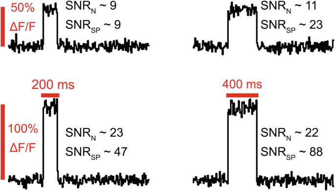

  

  Variation in SNR due to calculation method

• 2. The Fundamental Limit on SNR in Optical Imaging

  The physical nature of photon detection limits the theoretical maximum SNR of functional optical imaging. We measure the fluorescence intensity, F, of an indicator to infer something about the underlying physiological process it reports. Poisson noise due to a collection of fluorescence photons dictates how well we can do this for a given number of photons collected. The Poisson distribution gives the probability of detecting k photons in an interval when the mean rate is F₀ as

  $$ P\left(F=k|{F}_0\right)=\frac{e^{-{F}_0}{F}_0^k}{k!}. $$

  (12)

  Both the expected value and the variance of F are equal to F₀. Traces are commonly normalized to the mean intensity, F₀, enabling easier comparison of structures with a different labeling brightness, and the variance of the normalized variable, F∕F₀, can be simply calculated due to the linearity of the expectation value as σ² = 1∕F₀. We assume here that the change in brightness is small compared to the baseline brightness, such that the noise during and outside the signal period is the same. Our normalized signal, S, is given by ΔF∕F₀, the change in fluorescence brightness, and so our signal-to-noise ratio is given by

  $$ SNR=\frac{S}{\sigma }=\frac{\Delta F}{F_0}\sqrt{F_0}. $$

  (13)

  The figure above illustrates this by drawing samples from a Poisson distribution to simulate fluorescent signals. The rate is increased by 10% in the central samples, and the baseline brightness is 10000 counts/sample in the top trace, and only 1000 counts/sample in the bottom. This leads to an SNR clearly increased by a factor of $\approx \sqrt{10}\approx 3$ from the bottom to the top trace. On the right, a graph shows the theoretical maximum achievable SNR for a given brightness, for different relative changes in fluorescence from the signal of interest, ΔF∕F₀. This demonstration assumes our imaging system is Poisson noise-limited, which is typically true for bright fluorescent samples (Fig. 7).

  Fig. 7

  

  Demonstration of the effect of Poisson noise on SNR. Reproduced from [88], CC BY-SA 4.0. Inspired by [31]

References

Abdelfattah AS, Farhi SL, Zhao Y, Brinks D, Zou P, Ruangkittisakul A, Platisa J, Pieribone VA, Ballanyi K, Cohen AE, et al. (2016) A bright and fast red fluorescent protein voltage indicator that reports neuronal activity in organotypic brain slices. J Neurosci 36(8):2458–2472
Abdelfattah AS, Kawashima T, Singh A, Novak O, Liu H, Shuai Y, Huang Y-C, Campagnola L, Seeman SC, Yu J, et al. (2019) Bright and photostable chemigenetic indicators for extended in vivo voltage imaging. Science 365(6454):699–704
Acker CD, Yan P, Loew LM (2011) Single-voxel recording of voltage transients in dendritic spines. Biophysical Journal 101(2):L11–3
Adam Y, Kim JJ, Lou S, Zhao Y, Xie ME, Brinks D, Wu H, Mostajo-Radji MA, Kheifets S, Parot V, et al. (2019) Voltage imaging and optogenetics reveal behaviour-dependent changes in hippocampal dynamics. Nature 569(7756):413–417
Ahrens MB, Orger MB, Robson DN, Li JM, Keller PJ (2013) Whole-brain functional imaging at cellular resolution using light-sheet microscopy. Nature Methods 10(5):413
Aimon S, Katsuki T, Jia T, Grosenick L, Broxton M, Deisseroth K, Sejnowski TJ, Greenspan RJ (2019) Fast near-whole– brain imaging in adult Drosophila during responses to stimuli and behavior. PLoS Biology 17(2):e2006732
Akerboom J, Carreras Calderón N, Tian L, Wabnig S, Prigge M, Tolö J, Gordus A, Orger MB, Severi KE, Macklin JJ, et al. (2013) Genetically encoded calcium indicators for multi-color neural activity imaging and combination with optogenetics. Front Mol Neurosci 6:2
Anselmi F, Ventalon C, Bègue A, Ogden D, Emiliani V (2011) Three-dimensional imaging and photostimulation by remote-focusing and holographic light patterning. Proc Natl Acad Sci 108(49):19504–19509
Antic S, Zecevic D (1995) Optical signals from neurons with internally applied voltage-sensitive dyes. J Neurosci Offic J Soc Neurosci 15(2):1392–1405
Baker CA, Elyada YM, Parra A, Bolton MM (2016) Cellular resolution circuit mapping with temporal-focused excitation of soma-targeted channelrhodopsin. Elife 5:e14193
Bando Y, Sakamoto M, Kim S, Ayzenshtat I, Yuste R (2019) Comparative evaluation of genetically encoded voltage indicators. Cell Reports 26(3):802–813
Beaulieu DR, Davison IG, Kılıç K, Bifano TG, Mertz J (2020) Simultaneous multiplane imaging with reverberation two-photon microscopy. Nature Methods 17(3):283–286
Beck C, Zhang D, Gong Y (2019) Enhanced genetically encoded voltage indicators advance their applications in neuroscience. Curr Opin Biomed Eng 12:111–117
Berridge MJ, Lipp P, Bootman MD (2000) The versatility and universality of calcium signalling. Nat Rev Mol cell Biol 1(1):11–21
Bewersdorf J, Pick R, Hell SW (1998) Multifocal multiphoton microscopy. Optics Letters 23(9):655–657
Bindocci E, Savtchouk I, Liaudet N, Becker D, Carriero G, Volterra A (2017) Three-dimensional ca2+ imaging advances understanding of astrocyte biology. Science 356(6339):eaai8185
Bloodgood BL, Sabatini BL (2007) Ca2+ signaling in dendritic spines. Curr Opin Neurobiol 17(3):345–351
Blunck R, Chanda B, Bezanilla F (2005) Nano to micro-fluorescence measurements of electric fields in molecules and genetically specified neurons. J Membrane Biol 208(2):91–102
Botcherby EJ, Booth MJ, Juškaitis R, Wilson T (2008) Real-time extended depth of field microscopy. Optics Express 16(26):21843–21848. https://doi.org/10.1364/OE.16.021843. http://www.opticsexpress.org/abstract.cfm?URI=oe-16-26-21843
Bouchard MB, Voleti V, Mendes CS, Lacefield C, Grueber WB, Mann RS, Bruno RM, Hillman EMC (2015) Swept confocally-aligned planar excitation (scape) microscopy for high-speed volumetric imaging of behaving organisms. Nature Photonics 9(2):113
Bovetti S, Moretti C, Zucca S, Dal Maschio M, Bonifazi P, Fellin T (2017) Simultaneous high-speed imaging and optogenetic inhibition in the intact mouse brain. Scientific Reports 7:40041
Breuninger T, Greger K, Stelzer EHK (2007) Lateral modulation boosts image quality in single plane illumination fluorescence microscopy. Optics Letters 32(13):1938–1940
Castanares ML, Gautam V, Drury J, Bachor H, Daria VR (2016) Efficient multi-site two-photon functional imaging of neuronal circuits. Biomed Opt Exp 7(12):5325–5334
Chen JL, Voigt FF, Javadzadeh M, Krueppel R, Helmchen F (2016) Long-range population dynamics of anatomically defined neocortical networks. eLife 5:2221
Chen T-W, Wardill TJ, Sun Y, Pulver SR, Renninger SL, Baohan A, Schreiter ER, Kerr RA, Orger MB, Jayaraman V, et al. (2013) Ultrasensitive fluorescent proteins for imaging neuronal activity. Nature 499(7458):295–300
Cheng A, Gonçalves JT, Golshani P, Arisaka K, Portera-Cailliau C (2011) Simultaneous two-photon calcium imaging at different depths with spatiotemporal multiplexing. Nature Methods 8(2):139–142
Cong L, Wang Z, Chai Y, Hang W, Shang C, Yang W, Bai L, Du J, Wang K, Wen Q (2017) Rapid whole brain imaging of neural activity in freely behaving larval zebrafish (Danio rerio). eLife 6:60
Dana H, Marom A, Paluch S, Dvorkin R, Brosh I, Shoham S (2014) Hybrid multiphoton volumetric functional imaging of large-scale bioengineered neuronal networks. Nature Communications 5:3997
Dana H, Sun Y, Mohar B, Hulse BK, Kerlin AM, Hasseman JP, Tsegaye G, Tsang A, Wong A, Patel R, et al. (2019) High-performance calcium sensors for imaging activity in neuronal populations and microcompartments. Nature Methods 16(7):649–657
Denk W, Strickler JH, Webb WW (1990) Two-photon laser scanning fluorescence microscopy. Science 248:73–76
Djurisic M, Zochowski M, Wachowiak M, Falk CX, Cohen LB, Zecevic D (2003) Optical monitoring of neural activity using voltage-sensitive dyes. Methods Enzymol 361:423–451. ISSN:00766879. https://doi.org/10.1016/S0076-6879(03)61022-0. https://www.sciencedirect.com/science/article/pii/S0076687903610220
Ducros M, Houssen YG, Bradley J, de Sars V, Charpak S (2013) Encoded multisite two-photon microscopy. Proc Natl Acad Sci 110(32):13138–13143
Faisal AA, Selen LPJ, Wolpert DM (2008) Noise in the nervous system. Nat Rev Neurosci 9(4):292–303
Fan LZ, Kheifets S, Böhm UL, Wu H, Piatkevich KD, Xie ME, Parot V, Ha Y, Evans KE, Boyden ES, et al. (2020) All-optical electrophysiology reveals the role of lateral inhibition in sensory processing in cortical layer 1. Cell 180(3):521–535
Fernández A, Straw A, Distel M, Leitgeb R, Baltuska A, Verhoef AJ (2020) Dynamic real-time subtraction of stray-light and background for multiphoton imaging. Biomed Opt Exp 12(1):288. https://doi.org/10.1364/boe.403255
Forli A, Vecchia D, Binini N, Succol F, Bovetti S, Moretti C, Nespoli F, Mahn M, Baker CA, Bolton MM, et al. (2018) Two-photon bidirectional control and imaging of neuronal excitability with high spatial resolution in vivo. Cell Reports 22(11):3087–3098
Forli A, Pisoni M, Printz Y, Yizhar O, Fellin T (2021) Optogenetic strategies for high-efficiency all-optical interrogation using blue-light-sensitive opsins. eLife 10. https://doi.org/10.7554/eLife.63359
Foust AJ, Schei JL, Rojas MJ, Rector DM (2008) In vitro and in vivo noise analysis for optical neural recording. J Biomed Opt 13(4):044038
Foust AJ, Zampini V, Tanese D, Papagiakoumou E, Emiliani V (2015) Computer-generated holography enhances voltage dye fluorescence discrimination in adjacent neuronal structures. Neurophotonics 2(2):021007
Fu T, Arnoux I, Döring J, Backhaus H, Watari H, Stasevicius I, Fan W, Stroh A (2021) Exploring two-photon optogenetics beyond 1100 nm for specific and effective all-optical physiology. iScience 24(3):102184. https://doi.org/10.1016/j.isci.2021.102184. https://doi.org/10.1016/j.isci.2021.102184
Gonzalez JE, Tsien RY (1995) Voltage sensing by fluorescence resonance energy transfer in single cells. Biophysical Journal 69:1272–1280
Grienberger C, Konnerth A (2012) Imaging calcium in neurons. Neuron 73(5):862–885
Grosenick L, Broxton M, Kim CK, Liston C, Poole B, Yang S, Andalman A, Scharff E, Cohen N, Yizhar O, Ramakrishnan C, Ganguli S, Suppes P, Levoy M, Deisseroth K (2017) Identification of cellular-activity dynamics across large tissue volumes in the mammalian brain. bioRxiv. https://doi.org/10.1101/132688
Guo ZV, Hart AC, Ramanathan S (2009) Optical interrogation of neural circuits in Caenorhabditis elegans. Nature Methods 6(12):891
Hell SW, Bahlmann K, Schrader M, Soini A, Malak HM, Gryczynski I, Lakowicz JR (1996) Three-photon excitation in fluorescence microscopy. J Biomed Opt 1(1):71–74
Helmchen F, Denk W (2005) Deep tissue two-photon microscopy. Nature Methods 2(12):932–940
Hochbaum DR, Zhao Y, Farhi SL, Klapoetke N, Werley CA, Kapoor V, Zou P, Kralj JM, Maclaurin D, Smedemark-Margulies N, et al. (2014) All-optical electrophysiology in mammalian neurons using engineered microbial rhodopsins. Nature Methods 11(8):825
Hontani Y, Xia F, Xu C (2021) Multicolor three-photon fluorescence imaging with single-wavelength excitation deep in mouse brain. Science Advances 7(12):eabf3531. https://doi.org/10.1126/sciadv.abf3531
Hoover EE, Young MD, Chandler EV, Luo A, Field JJ, Sheetz KE, Sylvester AW, Squier JA (2011) Remote focusing for programmable multi-layer differential multiphoton microscopy. Biomed Opt Exp 2(1):113–122
Howe CL, Quicke P, Song P, Verinaz-Jadan H, Dragotti PL, Foust AJ (2022) Comparing synthetic refocusing to deconvolution for the extraction of neuronal calcium transients from light fields. Neurophotonics 9(4):041404
Huisken J, Swoger J, Del Bene F, Wittbrodt J, Stelzer EHK (2004) Optical sectioning deep inside live embryos by selective plane illumination microscopy. Science 305(5686):1007–1009
Jing M, Zhang P, Wang G, Feng J, Mesik L, Zeng J, Jiang H, Wang S, Looby JC, Guagliardo NA, et al. (2018) A genetically encoded fluorescent acetylcholine indicator for in vitro and in vivo studies. Nature Biotechnology 36(8):726–737
Kazemipour A, Novak O, Flickinger D, Marvin JS, Abdelfattah AS, King J, Borden PM, Kim JJ, Al-Abdullatif SH, Deal PE, et al. (2019) Kilohertz frame-rate two-photon tomography. Nature Methods 16(8):778
Keller PJ, Ahrens MB (2015) Visualizing whole-brain activity and development at the single-cell level using light-sheet microscopy. Neuron 85(3):462–483
Kim KH, Buehler C, Bahlmann K, Ragan T, Lee W-CA, Nedivi E, Heffer EL, Fantini S, So PTC (2007) Multifocal multiphoton microscopy based on multianode photomultiplier tubes. Optics Express 15(18):11658–11678
Kim MK, Lim CS, Hong JT, Han JH, Jang H-Y, Kim HM, Cho BR (2010) Sodium-ion-selective two-photon fluorescent probe for in vivo imaging. Angewandte Chemie Int Edn 49(2):364–367
Klapoetke NC, Murata Y, Kim SS, Pulver SR, Birdsey-Benson A, Cho YK, Morimoto TK, Chuong AS, Carpenter EJ, Tian Z, et al. (2014) Independent optical excitation of distinct neural populations. Nature Methods 11(3):338
Knöpfel T, Díez-García J, Akemann W (2006) Optical probing of neuronal circuit dynamics: genetically encoded versus classical fluorescent sensors. Trends Neurosci 29(3):160–166. ISSN:0166-2236. https://doi.org/10.1016/j.tins.2006.01.004. http://www.sciencedirect.com/science/article/pii/S0166223606000051
Kondo M, Kobayashi K, Ohkura M, Nakai J, Matsuzaki M (2017) Two-photon calcium imaging of the medial prefrontal cortex and hippocampus without cortical invasion. eLIFE 6:e26839
Kulkarni RU, Miller EW (2017) Voltage imaging: pitfalls and potential. Biochemistry 56(39):5171–5177
Lamy CM, Chatton J-Y (2011) Optical probing of sodium dynamics in neurons and astrocytes. Neuroimage 58(2):572–578
Lecoq J, Orlova N, Grewe BF (2019) Wide. fast. deep: Recent advances in multiphoton microscopy of in vivo neuronal activity. J Neurosci 39(46):9042–9052. https://doi.org/10.1523/jneurosci.1527-18.2019
Lim D, Mertz J, Chu KK (2008) Wide-field fluorescence sectioning with hybrid speckle and uniform-illumination microscopy. Optics Letters 33(16):1819–1821
Lim DH, Mohajerani MH, LeDue J, Boyd J, Chen S, Murphy TH (2012) In vivo large-scale cortical mapping using channelrhodopsin-2 stimulation in transgenic mice reveals asymmetric and reciprocal relationships between cortical areas. Front Neural Circuits 6:11
Lin JY, Knutsen PM, Muller A, Kleinfeld D, Tsien RY (2013) ReaChR: a red-shifted variant of channelrhodopsin enables deep transcranial optogenetic excitation. Nature Neuroscience 16(10):1499
Lu R, Sun W, Liang Y, Kerlin A, Bierfeld J, Seelig JD, Wilson DE, Scholl B, Mohar B, Tanimoto M, et al. (2017) Video-rate volumetric functional imaging of the brain at synaptic resolution. Nature Neuroscience 20(4):620
Mahn M, Gibor L, Patil P, Cohen-Kashi Malina K, Oring S, Printz Y, Levy R, Lampl I, Yizhar O (2018) High-efficiency optogenetic silencing with soma-targeted anion-conducting channelrhodopsins. Nature Communications 9(1):1–15
Manita S, Miyazaki K, Ross WN (2011) Synaptically activated Ca2+ waves and NMDA spikes locally suppress voltage-dependent ca2+ signalling in rat pyramidal cell dendrites. J Physiol 589(20):4903–4920
Marvin JS, Borghuis BG, Tian L, Cichon J, Harnett MT, Akerboom J, Gordus A, Renninger SL, Chen T-W, Bargmann CI, et al. (2013) An optimized fluorescent probe for visualizing glutamate neurotransmission. Nature Methods 10(2):162
Marvin JS, Scholl B, Wilson DE, Podgorski K, Kazemipour A, Müller JA, Schoch S, José Urra Quiroz F, Rebola N, Bao H, et al. (2018) Stability, affinity, and chromatic variants of the glutamate sensor iGluSnFR. Nature Methods 15(11):936–939
Marvin JS, Shimoda Y, Magloire V, Leite M, Kawashima T, Jensen TP, Kolb I, Knott EL, Novak O, Podgorski K, et al. (2019) A genetically encoded fluorescent sensor for in vivo imaging of GABA. Nature Methods, p. 1
McMahon SM, Jackson MB (2018) An inconvenient truth: calcium sensors are calcium buffers. Trends Neurosci 41(12):880–884
Mertz J, Kim J (2010) Scanning light-sheet microscopy in the whole mouse brain with HiLo background rejection. J Biomed Opt 15(1):016027
Miyazaki K, Manita S, Ross WN (2012) Developmental profile of localized spontaneous ca2+ release events in the dendrites of rat hippocampal pyramidal neurons. Cell Calcium 52(6):422–432
Murakami T, Yoshida T, Matsui T, Ohki K (2015) Wide-field ca2+ imaging reveals visually evoked activity in the retrosplenial area. Front Mol Neurosci 8:20
Neil MAA, Juškaitis R, Wilson T (1997) Method of obtaining optical sectioning by using structured light in a conventional microscope. Optics Letters 22(24):1905–1907
Ng R, Adams A, Footer M, Horowitz M, Levoy M (2006) Light field microscopy. ACM Trans Graph 25(3):924–934
Nielsen T, Fricke M, Hellweg D, Andresen P (2001) High efficiency beam splitter for multifocal multiphoton microscopy. J Microscopy 201(3):368–376
Nikolenko V, Watson BO, Araya R, Woodruff A, Peterka DS, Yuste R (2008) SLM microscopy: scanless two-photon imaging and photostimulation using spatial light modulators. Front Neural Circuits 2:5
Nobauer T, Skocek O, Pernia-Andrade AJ, Weilguny L, Traub FM, Molodtsov MI, Vaziri A (2017) Video rate volumetric Ca2+ imaging across cortex using seeded iterative demixing (SID) microscopy. Nature Methods 14(8):811–818
Olarte OE, Andilla J, Artigas D, Loza-Alvarez P (2015) Decoupled illumination detection in light sheet microscopy for fast volumetric imaging. Optica 2(8):702
Oron D, Tal E, Silberberg Y (2005) Scanningless depth-resolved microscopy. Optics Express 13(5):1468–1476
Packer AM, Russell LE, Dalgleish HWP, Häusser M (2014) Simultaneous all-optical manipulation and recording of neural circuit activity with cellular resolution in vivo. Nature Methods 12(2):140–146. https://doi.org/10.1038/nmeth.3217
Pégard NC, Liu H-Y, Antipa N, Gerlock M, Adesnik H, Waller L (2016) Compressive light-field microscopy for 3d neural activity recording. Optica 3(5):517–524
Pozzi P, Gandolfi D, Tognolina M, Chirico G, Mapelli J, D’Angelo E (2015) High-throughput spatial light modulation two-photon microscopy for fast functional imaging. Neurophotonics 2(1):015005
Prevedel R, Yoon Y-G, Hoffmann M, Pak N, Wetzstein G, Kato S, Schrödel T, Raskar R, Zimmer M, Boyden ES, Vaziri A (2014) Simultaneous whole-animal 3D imaging of neuronal activity using light-field microscopy. Nature Methods 11(7):727–730
Prevedel R, Verhoef AJ, Pernia-Andrade AJ, Weisenburger S, Huang BS, Nöbauer T, Fernández A, Delcour JE, Golshani P, Baltuska A, et al. (2016) Fast volumetric calcium imaging across multiple cortical layers using sculpted light. Nature Methods 13(12):1021–1028
Quicke P (2019) Improved methods for functional neuronal imaging with genetically encoded voltage indicators. PhD thesis, Imperial College, London
Quicke P, Reynolds S, Neil M, Knöpfel T, Schultz SR, Foust AJ (2018) High speed functional imaging with source localized multifocal two-photon microscopy. Biomed Opt Exp 9(8):3678–3693
Quicke P, Song C, McKimm EJ, Milosevic MM, Howe CL, Neil M, Schultz SR, Antic SD, Foust AJ, Knöpfel T (2019) Single-neuron level one-photon voltage imaging with sparsely targeted genetically encoded voltage indicators. Front Cell Neurosci 13:39. ISSN:1662-5102. https://doi.org/10.3389/fncel.2019.00039. https://www.frontiersin.org/article/10.3389/fncel.2019.00039
Quicke P, Howe CL, Song P, Jadan HV, Song C, Knöpfel T, Neil M, Dragotti PL, Schultz SR, Foust AJ (2020) Subcellular resolution three-dimensional light-field imaging with genetically encoded voltage indicators. Neurophotonics 7(3):035006. https://doi.org/10.1117/1.nph.7.3.035006
Quirin S, Vladimirov N, Yang C-T, Peterka DS, Yuste R, Ahrens MB (2016) Calcium imaging of neural circuits with extended depth-of-field light-sheet microscopy. Optics Letters 41(5):855–858
Raimondo JV, Irkle A, Wefelmeyer W, Newey SE, Akerman CJ (2012) Genetically encoded proton sensors reveal activity-dependent ph changes in neurons. Front Mol Neurosci 5:68
Raimondo JV, Joyce B, Kay L, Schlagheck T, Newey SE, Srinivas S, Jon Akerman C (2013) A genetically-encoded chloride and ph sensor for dissociating ion dynamics in the nervous system. Front Cell Neurosci 7:202
Rose T, Goltstein PM, Portugues R, Griesbeck O (2014) Putting a finishing touch on GECIs. Front Mol Neurosci 7:88
Rowlands CJ, Park D, Bruns OT, Piatkevich KD, Fukumura D, Jain RK, Bawendi MG, Boyden ES, So PTC (2017) Wide-field three-photon excitation in biological samples. Light Sci Appl 6(5):e16255–e16255
Schrödel T, Prevedel R, Aumayr K, Zimmer M, Vaziri A (2013) Brain-wide 3d imaging of neuronal activity in Caenorhabditis elegans with sculpted light. Nature Methods 10(10):1013
Shao Y, Qu J, Peng X, Niu H, Qin W, Liu H, Gao BZ (2012) Addressable multiregional and multifocal multiphoton microscopy based on a spatial light modulator. J Biomed Opt 17(3):030505
Shemesh OA, Tanese D, Zampini V, Linghu C, Piatkevich K, Ronzitti E, Papagiakoumou E, Boyden ES, Emiliani V (2017) Temporally precise single-cell-resolution optogenetics. Nature Neuroscience 20(12):1796–1806
Skocek O, Nobauer T, Weilguny L, Martínez Traub F, Xia CN, Molodtsov MI, Grama A, Yamagata M, Aharoni D, Cox DD, Golshani P, Vaziri A (2018) High-speed volumetric imaging of neuronal activity in freely moving rodents. Nature Methods 15(6):429–432
Smith SL (2019) Building a two-photon microscope is easy. In: E Hartveit (ed), Multiphoton microscopy, pp 1–16. Springer, New York
Sofroniew NJ, Flickinger D, King J, Svoboda K (2016) A large field of view two-photon mesoscope with subcellular resolution for in vivo imaging. Elife 5:e14472
Song A, Charles AS, Koay SA, Gauthier JL, Thiberge SY, Pillow JW, Tank DW (2017) Volumetric two-photon imaging of neurons using stereoscopy (vTwINS). Nature Methods 14(4):420–426
Soor NS, Quicke P, Howe CL, Pang KT, Neil MAA, Schultz SR, Foust AJ (2019) All-optical crosstalk-free manipulation and readout of chronos-expressing neurons. J Phys D Appl Phys 52(10):104002
Steinmetz NA, Buetfering C, Lecoq J, Lee CR, Peters AJ, Jacobs EAK, Coen P, Ollerenshaw DR, Valley MT, De Vries SEJ, et al. (2017) Aberrant cortical activity in multiple GCaMP6-expressing transgenic mouse lines. eNeuro. https://doi.org/10.1523/ENEURO.0207-17.2017
Stirman JN, Smith IT, Kudenov MW, Smith SL (2016) Wide field-of-view, multi-region, two-photon imaging of neuronal activity in the mammalian brain. Nature Biotechnology 34(8):857
Szabo V, Ventalon C, De Sars V, Bradley J, Emiliani V (2014) Spatially selective holographic photoactivation and functional fluorescence imaging in freely behaving mice with a fiberscope. Neuron 84(6):1157–1169
Takahara Y, Matsuki N, Ikegaya Y (2011) Nipkow confocal imaging from deep brain tissues. J Integrat Neurosci 10(01):121–129
Tanese D, Weng J-Y, Zampini V, de Sars V, Canepari M, Rozsa BJ, Emiliani V, Zecevic D (2017) Imaging membrane potential changes from dendritic spines using computer-generated holography. Neurophotonics 4(3):031211
Therrien OD, Aubé B, Pagès S, De Koninck P, Côté D (2011) Wide-field multiphoton imaging of cellular dynamics in thick tissue by temporal focusing and patterned illumination. Biomed Opt Exp 2(3):696–704
Thung K, Raveendran P (2009) A survey of image quality measures. In: 2009 International conference for technical postgraduates (TECHPOS), pp 1–4
Tian L, Hires SA, Mao T, Huber D, Chiappe ME, Chalasani SH, Petreanu L, Akerboom J, McKinney SA, Schreiter ER, et al. (2009) Imaging neural activity in worms, flies and mice with improved GCaMP calcium indicators. Nature Methods 6(12):875
Tomer R, Lovett-Barron M, Kauvar I, Andalman A, Burns VM, Sankaran S, Grosenick L, Broxton M, Yang S, Deisseroth K (2015) SPED light sheet microscopy: fast mapping of biological system structure and function. Cell 163(7):1796–1806
Tsuda S, Kee MZL, Cunha C, Kim J, Yan P, Loew LM, Augustine GJ (2013) Probing the function of neuronal populations: combining micromirror-based optogenetic photostimulation with voltage-sensitive dye imaging. Neuroscience Research 75(1):76–81
van Drongelen W (2007) Signal processing for neuroscientists: Introduction to the analysis of physiological signals. J Motor Behav 39(2):158
Venkatachalam V, Cohen AE (2014) Imaging GFP-based reporters in neurons with multiwavelength optogenetic control. Biophys J 107(7):1554–1563
Villette V, Chavarha M, Dimov IK, Bradley J, Pradhan L, Mathieu B, Evans SW, Chamberland S, Shi D, Yang R, et al. (2019) Ultrafast two-photon imaging of a high-gain voltage indicator in awake behaving mice. Cell 179(7):1590–1608
Weisenburger S, Tejera F, Demas J, Chen B, Manley J, Sparks FT, Traub FM, Daigle T, Zeng H, Losonczy A, et al. (2019) Volumetric ca2+ imaging in the mouse brain using hybrid multiplexed sculpted light microscopy. Cell 177(4):1050–1066
Willadt S, Canepari M, Yan P, Loew LM, Vogt KE (2014) Combined optogenetics and voltage sensitive dye imaging at single cell resolution. Front Cell Neurosci 8:311
Wu J, Liang Y, Chen S, Hsu C-L, Chavarha M, Evans SW, Shi D, Lin MZ, Tsia KK, Ji N (2020) Kilohertz two-photon fluorescence microscopy imaging of neural activity in vivo. Nature Methods 17(3):287–290
Xu C, Zipfel W, Shear JB, Williams RM, Webb WW (1996) Multiphoton fluorescence excitation: new spectral windows for biological nonlinear microscopy. Proc Natl Acad Sci USA 93(20):10763–10768
Yang SJ, Allen WE, Kauvar I, Andalman AS, Young NP, Kim CK, Marshel JH, Wetzstein G, Deisseroth K (2015) Extended field-of-view and increased-signal 3d holographic illumination with time-division multiplexing. Optics Express 23(25):32573–32581
Yang W, Miller J-EK, Carrillo-Reid L, Pnevmatikakis E, Paninski L, Yuste R, Peterka DS (2016) Simultaneous multi-plane imaging of neural circuits. Neuron 89(2):269–284
Yang W, Carrillo-Reid L, Bando Y, Peterka DS, Yuste R (2018) Simultaneous two-photon imaging and two-photon optogenetics of cortical circuits in three dimensions. Elife 7:e32671
Yizhar O, Fenno LE, Prigge M, Schneider F, Davidson TJ, O’shea DJ, Sohal VS, Goshen I, Finkelstein J, Paz JT, et al. (2011) Neocortical excitation/inhibition balance in information processing and social dysfunction. Nature 477(7363):171–178
Yoshida E, Terada S-I, Tanaka YH, Kobayashi K, Ohkura M, Nakai J, Matsuzaki M (2018) In vivo wide-field calcium imaging of mouse thalamocortical synapses with an 8 k ultra-high-definition camera. Scientific Reports 8(1):1–15
Zhang T, Hernandez O, Chrapkiewicz R, Shai A, Wagner MJ, Zhang Y, Wu C-H, Li JZ, Inoue M, Gong Y, et al. (2019) Kilohertz two-photon brain imaging in awake mice. Nature Methods 16(11):1119–1122
Zhu G, Van Howe J, Durst M, Zipfel W, Xu C (2005) Simultaneous spatial and temporal focusing of femtosecond pulses. Optics express 13(6):2153–2159
Zinter JP, Levene MJ (2011) Maximizing fluorescence collection efficiency in multiphoton microscopy. Optics Express 19(16):15348–15362
Zipfel WR, Williams RM, Webb WW (2003) Nonlinear magic: multiphoton microscopy in the biosciences. Nature Biotechnology 21(11):1369–1377
Acknowledgements
This work was supported by the Biotechnology and Biological Sciences Research Council (BB/R009007/1), the Royal Academy of Engineering under the RAEng Research Fellowships scheme (RF1415/14/26), and the Engineering and Physical Sciences Research Council (EP/L016737/1).
Author information
Authors and Affiliations
Corresponding author
Editor information
Editors and Affiliations
Rights and permissions
Open Access This chapter is licensed under the terms of the Creative Commons Attribution 4.0 International License (http://creativecommons.org/licenses/by/4.0/), which permits use, sharing, adaptation, distribution and reproduction in any medium or format, as long as you give appropriate credit to the original author(s) and the source, provide a link to the Creative Commons license and indicate if changes were made.
The images or other third party material in this chapter are included in the chapter's Creative Commons license, unless indicated otherwise in a credit line to the material. If material is not included in the chapter's Creative Commons license and your intended use is not permitted by statutory regulation or exceeds the permitted use, you will need to obtain permission directly from the copyright holder.
Copyright information
© 2023 The Author(s)
About this protocol
Cite this protocol
Quicke, P., Howe, C.L., Foust, A.J. (2023). Balancing the Fluorescence Imaging Budget for All-Optical Neurophysiology Experiments. In: Papagiakoumou, E. (eds) All-Optical Methods to Study Neuronal Function. Neuromethods, vol 191. Humana, New York, NY. https://doi.org/10.1007/978-1-0716-2764-8_2
Download citation
DOI: https://doi.org/10.1007/978-1-0716-2764-8_2
Published:
Publisher Name: Humana, New York, NY
Print ISBN: 978-1-0716-2763-1
Online ISBN: 978-1-0716-2764-8
eBook Packages: Springer Protocols