Novel Parametric Circuit Modeling for Li-Ion Batteries

Abstract

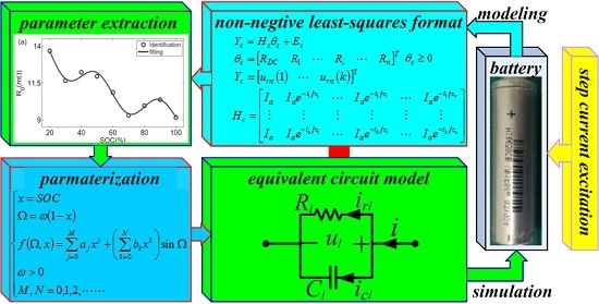
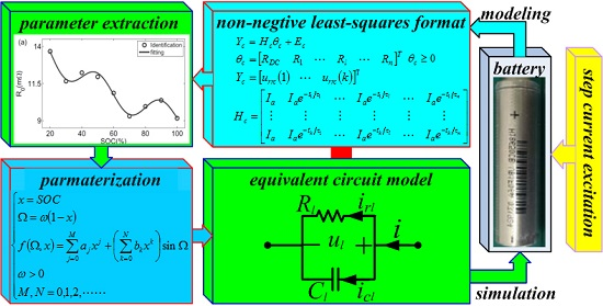
Because of their simplicity and dynamic response, current pulse series are often used to extract parameters for equivalent electrical circuit modeling of Li-ion batteries. These models are then applied for performance simulation, state estimation, and thermal analysis in electric vehicles. However, these methods have two problems: The assumption of linear dependence of the matrix columns and negative parameters estimated from discrete-time equations and least-squares methods. In this paper, continuous-time equations are exploited to construct a linearly independent data matrix and parameterize the circuit model by the combination of non-negative least squares and genetic algorithm, which constrains the model parameters to be positive. Trigonometric functions are then developed to fit the parameter curves. The developed model parameterization methodology was applied and assessed by a standard driving cycle.

1. Introduction

With price reductions and safety improvements, Li-ion batteries are increasingly being used to power electric vehicles [1]. Battery modeling is vital to fuel economy simulation and system control of electrified vehicles in that: batteries are the onboard power source of electrical devices; reliable and efficient battery models can maximize performance of these devices; and battery package size and cost should be evaluated by battery models.

Equivalent electrical circuit (EEC) is one of most commonly used techniques to model Li-ion batteries for electric vehicles, the popular topology of which consists of one resistor, one or multiple resistor-capacitor (RC) pairs, and one electromotive force in series [2]. This EEC can be expressed through succinct ordinary differential equations. Moreover, that the number of RC pairs either increases or decreases makes the EEC flexible to battery modeling for varying applications such as overall performance simulation of electric vehicles, real-time control, and analysis of battery transient response. In this battery circuit model, the electromotive force relates to the amount of Li-ion, usually called the open-circuit voltage (OCV), which is a function of the state-of-charge (SOC), temperature, and lifetime. The serial resistor denotes an ohmic voltage drop when a current flows through the battery terminal taps, current collectors, electrode material, electrolyte, and separator.

Any electrochemical reaction undergoes activation polarization and concentration polarization [3]. Compared to other electrochemical batteries, Li-ion batteries have similar polarization effects caused by charge transfer, double-layer capacitance, and ion-concentration gradient, related over-potentials of which can be represented by voltage drops of the battery current flowing through the RC pairs. However, compared to lead-acid and NiMH batteries, Li-ion batteries always form a solid electrolyte interface (SEI) layer between the graphite anode and electrolytes at their first charge cycle [4]. The thickness increase of the SEI layer can consume Li-ion and may have a negative influence on Li-ion transport, which can lead to capacity decrease and performance degradation of Li-ion batteries [5]. In order to characterize the behavior of the SEI layer, either one or more RC pairs in series have been used to build a relationship between the formation voltage and growth of the SEI layer [6,7].

Parameter extraction is a significant concern for an EEC model fitted to a Li-ion battery because the RC-pair parameters are not measurable and model parameters change with working conditions. There are many optimization algorithms for parameter estimation of battery EEC models, including least-squares (LS) [8,9,10,11], Kalman filter [12,13], genetic algorithm [14], sequential quadratic programming [15], and swarm optimization [16]. By adjusting the model parameters, these optimization algorithms minimize error between each experimental battery voltage dataset and the corresponding simulated results.

For these numerical optimizers, it is difficult to separate RC-pair parameters and avoid negative parameters. One problem comes from the same voltage of the RC pairs on the EEC. For this problem, Jackey et al. [17] used a layer technique together with a gradient-based optimizer to extract RC-pair parameters. For the other problem about the negative parameters, the numerical optimizers get the simulated battery voltages approximated to the measurements, by which the values of the resistor and capacitor of one RC pair can be less than 0 if there are no corresponding constraints inserted into the optimizers. It becomes evident when the number of RC pairs is greater than 1 and increases. Because the RC pairs of an EEC relate to the charge transfer, double-layer effect, concentration diffusion, and SEI layer growth of a specific Li-ion battery, it is plausible for negative resistances and capacitances to characterize these physical-chemistry behaviors, although the negative circuit parameters are effective in mathematics. Hence, it is essential to use parameter optimizers confined by the boundary conditions of an EEC model’s positive parameters. However, there are few studies in the literature that address this issue.

The pulse series of battery current is often used as a test signal to extract parameters of the EECs of Li-ion batteries owing to both available multiple SOC values and corresponding transient response. There are several kinds of pulse curves, including hybrid power pulse cycle (HPPC) [14], equal-amplitude pulse series [8,18,19], and variable-amplitude pulse series [20,21]. Each current pulse and the corresponding voltage response data can be applied for parameter extraction of a battery EEC model during the non-zero current zone and/or relaxation period. However, it is probable to form linearly dependent row and column elements of an optimizer matrix during the equal-amplitude current period. For a commonly used LS method, there are two column elements of a data matrix to be linearly dependent in the formation of the normal equation. This issue also needs to be avoided for parameter estimators.

The main objective of this paper is to exploit a new estimator, the non-negative least-squares (NNLS) method for parameter estimation of an EEC model for a Li-ion battery. This parameter estimator is built on a newly developed normal equation, any matrix rows and columns of which are linearly independent. The paper is organized as follows: Section 2 presents the parameter extraction and model parameterization, Section 3 describes the test setup, Section 4 validates the modeling method, and Section 5 presents conclusions.

2. Battery Modeling

Mathematic expressions of the battery EEC model were developed to form the normal equations of the general LS method, the method of which was newly built based on the current equal-amplitude pulse series for linearly independent row and column elements of an optimizer matrix. Next, the NNLS method was first used to construct the parameter estimator of the battery EEC model. Finally, the genetic algorithm (GA) and NNLS were combined to estimate model parameters.

2.1. Basic Equations for Model Parameter Estimation

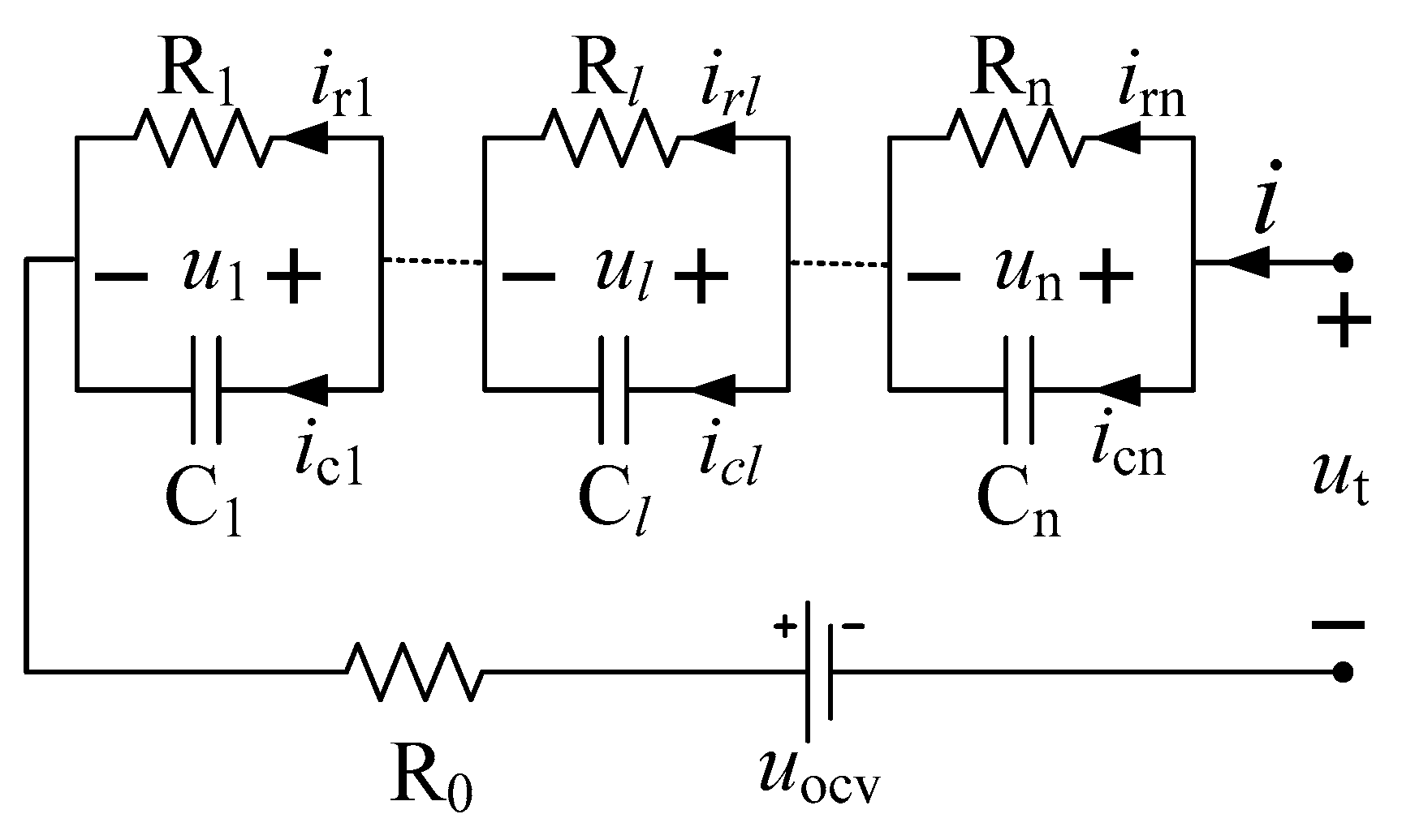
The schematic of the general EEC is used to model Li-ion batteries as shown in Figure 1, the discrete-time equations of which can be carried out by the Euler and bilinear transform [8,22]. In this circuit, multiple RC pairs characterize polarization effects of Li-ion batteries related to electrochemical behaviors such as charge transfer, double-layer effect, concentration gradient, and SEI layer growth. The mathematical model for the multiple RC-pair EEC in Figure 1 can be expressed in the following differential equations:

$$\{\begin{array}{l}{\dot{u}}_l=\left(-u_l+R_{l}i\right)/{\mathsf{\tau }}_l\\ u_t=u_{\mathrm{ocv}}+R_{0}i+{\displaystyle \sum _{l=1}^n{u}_l}\\ {\mathsf{\tau }}_l=R_l{C}_l\\ u_{\mathrm{ocv}}=f\left(SOC,T,L\right)\end{array}$$

(1)

where τ_l denotes the time constant of an RC pair, T denotes the battery operation temperature, and L denotes the battery life time. u_OCV, R₀, R_l, and C_l represent the battery OCV, ohmic resistance, polarization resistance, and capacitance, respectively.

If the battery is operated under constant temperature, $\partial u_{\text{ocv}}/\partial T=0$. An operation period of parameter extraction for the battery modeling can be assumed to be limited and much shorter than the battery lifetime. Hence, $\partial u_{\text{ocv}}/\partial L\approx 0$.

According to Equation (1), the transfer function of any RC pair in Figure 1 can be written as:

$$\frac{U_l\left(s\right)}{I\left(s\right)}=\frac{R_l}{1+{\mathsf{\tau }}_{l}s}$$

(2)

If u_ocv is known ahead of time, the impedance voltage u_rrc can be defined as:

$$u_{\text{rrc}}\left(t\right)=u_t\left(t\right)-u_{\text{OCV}}\left(t\right)$$

(3)

Supposing that the battery remains in a state of thermodynamic balance before the test signal is loaded, elements of the battery equivalent circuit can be at zero state, and the voltage response resulting from the step battery current can be provided by Equation (2) as:

$$U_{\text{rrc}}\left(s\right)=\left(R_0+{\displaystyle \sum _{l=1}^n\frac{R_l}{1+{\mathsf{\tau }}_{l}s}}\right)\frac{I_a}{s}$$

(4)

where I_a is the current amplitude of the step input.

The corresponding voltage-time function is given as:

$$u_{\text{rrc}}\left(t\right)=\left(R_{\text{DC}}+{\displaystyle \sum _{l=1}^n{R}_l{e}^{-t/{\mathsf{\tau }}_l}}\right)I_a$$

(5)

where R_DC denotes the total direct resistance of the Li-ion battery expressed as:

$$R_{\text{DC}}=R_0+{\displaystyle \sum _{l=1}^n{R}_l}$$

(6)

When battery voltage and current are sampled at time t_k (k = 1, 2, 3, …), the general LS format of Equation (5) can be written as:

$$Z=H\mathsf{\theta }+E$$

(7)

where E is the white noise vector and n is the number of RC pairs in Figure 1.

$$\mathsf{\theta }={\left[\begin{array}{cccccc}{R}_{DC}& R_1& \cdots & R_l& \cdots & R_n\end{array}\right]}^{\mathrm{T}}$$

$$Z={\left[\begin{array}{ccccc}{u}_{rrc}\left(1\right)& \cdots & u_{rrc}\left(r\right)& \cdots & u_{rrc}\left(k\right)\end{array}\right]}^{\mathrm{T}}$$

$$H=I_a^{n+1}\left[\begin{array}{cccccc}1& e^{-t_1/{\mathsf{\tau }}_1}& \cdots & e^{-t_r/{\mathsf{\tau }}_l}& \cdots & e^{-t_k/{\mathsf{\tau }}_n}\\ ⋮& ⋮& \cdots & ⋮& \cdots & ⋮\\ 1& e^{-t_r/{\mathsf{\tau }}_1}& \cdots & e^{-t_r/{\mathsf{\tau }}_l}& \cdots & e^{-t_k/{\mathsf{\tau }}_n}\\ ⋮& ⋮& \cdots & ⋮& \cdots & ⋮\\ 1& e^{-t_k/{\mathsf{\tau }}_1}& \cdots & e^{-t_r/{\mathsf{\tau }}_l}& \cdots & e^{-t_k/{\mathsf{\tau }}_n}\end{array}\right]$$

$$E={\left[\begin{array}{ccccc}e\left(1\right)& \cdots & e_l\left(k\right)& \cdots & e\left(k\right)\end{array}\right]}^T$$

and

$$1\le l\le n,n\ge 1$$

$$1<r<k,k\ge n+1$$

A cost function is used to minimize the square-error sum between measurements and simulations of the battery voltage.

$$J=\underset{s.t.{\mathsf{\theta }}^{*}>0}{\min }{\displaystyle \sum _{k=1}^n{\left[V_{t,m}\left(k\right)-V_{t,s}^{*}\left(k\right)\right]}^2}$$

(8)

where θ* is the identified parameter vector, and the sign of θ* > 0 means every elements of θ* larger than zero. The battery voltage is collected or stored at the kth step, V_t,m(k) for the measurement value, and V_t,s*(k) for the estimation.

According to this cost function (8), a normal equation can be derived from Equation (7).

$$\left(H^{T}H\right){\mathsf{\theta }}^{*}=H^{T}Z$$

(9)

When the battery is excited by the step current signal, either rows or columns of the matrix H of Equation (9) are linearly independent at different times t₁, …, t_k. The matrix of (H^TH) is non-singular, so the LS solution can be given by:

$${\mathsf{\theta }}^{*}={\left(H^{T}H\right)}^{-1}{H}^{T}Z$$

(10)

For an equal-amplitude current pulse series, any two column/row elements of each matrix in the developed normal equation for the LS solution are so linearly independent that the developed parameter estimator is divergent. However, there can be two linearly dependent columns in this normal equation of the general LS method, as shown in

Table 1. Comparison of normal equations between the general LS and developed LS methods.

Items	General LS Method [8,10,22]	Developed LS Method
Mechanismequations	$U_{\text{rrc}}\left(z^{-1}\right)=\left(R_0+{\displaystyle \sum _{l=1}^n\frac{b_0+b_1{z}^{-1}}{1+a_1{z}^{-1}}}\right)I\left(z^{-1}\right)$**	$U_{\text{rrc}}\left(s\right)=\left(R_0+\frac{R_l}{1+{\mathsf{\tau }}_l{z}^{-1}}\right)\frac{I_a}{s}$
Normal equations of LS	$\left(H^{T}H\right)\mathsf{\theta }=H^{T}Z$
	$H=\left[\begin{array}{ccccccc}{u}_{\text{rrc}}\left(n+1\right)& \cdots & u_{\text{rrc}}\left(l\right)& \cdots & u_{\text{rrc}}\left(1\right)& i\left(1\right)& i\left(0\right)\\ ⋮& \cdots & ⋮& \cdots & ⋮& ⋮& ⋮\\ u_{\text{rrc}}\left(n+r+1\right)& \cdots & u_{\text{rrc}}\left(l+r\right)& \cdots & u_{\text{rrc}}\left(r\right)& i\left(r\right)& i\left(r-1\right)\\ ⋮& \cdots & ⋮& \cdots & ⋮& ⋮& ⋮\\ u_{\text{rrc}}\left(n+k+1\right)& \cdots & u_{\text{rrc}}\left(l+k\right)& \cdots & u_{\text{rrc}}\left(k\right)& i\left(k\right)& i\left(k-1\right)\end{array}\right]$	$\begin{array}{l}H=I_a^{n+1}\\ \left[\begin{array}{cccccc}1& e^{-t_1/{\mathsf{\tau }}_1}& \cdots & e^{-t_r/{\mathsf{\tau }}_l}& \cdots & e^{-t_k/{\mathsf{\tau }}_n}\\ ⋮& ⋮& \cdots & ⋮& \cdots & ⋮\\ 1& e^{-t_r/{\mathsf{\tau }}_1}& \cdots & e^{-t_r/{\mathsf{\tau }}_l}& \cdots & e^{-t_k/{\mathsf{\tau }}_1}\\ ⋮& ⋮& \cdots & ⋮& \cdots & ⋮\\ 1& e^{-t_k/{\mathsf{\tau }}_1}& \cdots & e^{-t_r/{\mathsf{\tau }}_l}& \cdots & e^{-t_k/{\mathsf{\tau }}_1}\end{array}\right]\end{array}$
Dis-advantages	The last two column elements of the matrix H can be linearly dependent when equal-amplitude current pulses are excited to a battery. The data of H is sensitive to measurement noises.	Limited for an equal-amplitude current pulse series.
Advantages	Random-amplitude current excitation.	Any two column and row elements of the matrix H are linearly independent and robust to measurement noises.

** Note: b₀, b₁, and a₁ relate to the RC pair parameters and change with different discrete transforms, b₀ = 0 for the forward Euler transform, b₁ = 0 for the backward Euler transform, and both b₀ and b₁ are unequal to zero for the bilinear transform.

.

2.2. Non-Negative Parameter Identification Algorithm

By the general LS solution of Equation (10), the estimated parameters of the battery EEC model can be negative. This problem can be solved by an active set algorithm called non-negative least-squares (NNLS) [23]. Assuming that time constants of the RC pairs are known in the matrix H, the developed algorithm can be stated in

Table 2. NNLS algorithm for the parameter estimation of the EEC model of the Li-ion battery.

Step	Description
Initialization	$P=\varnothing$, $Q=\left\{\begin{array}{ccc}1& \cdots & n+1\end{array}\right\}$, ${\mathsf{\theta }}^{*}={\left[\begin{array}{ccccc}0& \cdots & 0& \cdots & 0\end{array}\right]}^{\mathrm{T}}$.
Iteration	(1): Set $w=H^T\left(Z-H{\mathsf{\theta }}^{*}\right)$. (2): If the set Q is empty or if $w_j\le 0$ for all $j\in Q$, go to End. (3): Find an index $m\in Q$ such that $w_m=\max \left(w_j:j\in Q\right)$. (4): Move the index m from the set Q to set P. (5): Define a $k\times \left(n+1\right)$ matrix : $$\text{Column\hspace{0.17em}of\hspace{0.17em}}{H}_P=\{\begin{array}{l}\text{column\hspace{0.17em}of\hspace{0.17em}}H\text{\hspace{0.17em}if\hspace{0.17em}}j\in P\\ 0\text{\hspace{0.17em}if\hspace{0.17em}}j\in Q\end{array}.$$ Compute the n-vector X as a solution of the least-squares problem $H_{P}X=Z$. Note that only the components $\left\{X_j,j\in P\right\}$ are determined by this problem. Define $\left\{X_j=0,j\in Q\right\}$. $$X={\left[{\left(H_P\right)}^T{H}_P\right]}^{-1}{\left(H_P\right)}^{T}Z.$$ (6): If $X_j>0$ for all $j\in P$, set ${\mathsf{\theta }}^{*}=X$ and go to Step 1. (7): Find an index $q\in P$, $\mathsf{\alpha }={\mathsf{\theta }}_q^{*}/\left({\mathsf{\theta }}_q^{*}-X_q\right)$, such that $$\mathsf{\alpha }=\min \left[{\mathsf{\theta }}_j^{*}/\left({\mathsf{\theta }}_j^{*}-X_j\right):X_j\le 0,j\in P\right].$$ (8): Set ${\mathsf{\theta }}^{*}={\mathsf{\theta }}^{*}+\mathsf{\alpha }\left(X-{\mathsf{\theta }}^{*}\right)$. (9): Move from the set P to set Q all indices $j\in P$ for which $X_j=0$. Go to Step 6.
End	All non-negative parameters of the battery EEC model are obtained.

for the parameter identification problem of Equations (7) and (8).

The GA is used with the cost function (8) to determine the RC-pair time constants. Each RC pair is set a time constant zone, the optimum value of which is found by using the GA. Once the time constants are set, the NNLS will be used to estimate the model resistances. This combination algorithm consists of two loops. The main loop is the GA for the estimated time constants, and the inner loop is the NNLS to identify resistances of the EEC. When estimated time constants and resistances make the simulated voltage most approximate to the voltage measurements, the mole parameters are determined. The combination algorithm is carried out by the GA solver gatool() and function lsqnonneg() of the Matlab/Simulink^® software (Mathworks, Natick, MA, USA).

2.3. Parameterization of Battery Circuit Models

Except for lookup tables, varying functions can be used to parameterize the EEC model of Li-ion batteries under working conditions such as SOC, temperature, and C-rate. For the SOC effects on model parameters, linear, quadratic, and exponent functions were used to parameterize the circuit model [8,17,22]. To establish the relationship between the polarization resistance and battery current, a logarithm function based on the Butler-Volmer equation for the one-RC-pair circuit was built [24]. However, there was no definite relationship between the capacitance and C-rate for battery model parameterization. At room temperature, these model parameters are considered to be affected by both SOC and C-rate. A unified trigonometric function polynomial was developed to fit each element parameter of the battery circuit model related to either the SOC or C-rate as given below.

$$\{\begin{array}{l}x=SOC\\ \mathsf{\Omega }=\mathsf{\omega }\left(1-x\right)\\ f\left(\mathsf{\Omega },x\right)={\displaystyle \sum _{j=0}^M{c}_j{x}^j}+\left({\displaystyle \sum _{k=0}^N{d}_k{x}^k}\right)\sin \mathsf{\Omega }\\ \mathsf{\omega }>0\\ M,N=0,1,2,\cdots \cdots \end{array}$$

(11)

where c_j and d_k denote the coefficients of the trigonometric function polynomial.

Each parameter of the battery circuit model is a function of both SOC and C-rate, which is the multiplication of the baseline parameter and current-dependency parameter ratio.

$$F_p\left(\mathsf{\Omega },x\right)=f_b\left(\mathsf{\Omega },x\right)\mathsf{\lambda }\left(f_r\left(\mathsf{\Omega },x\right)\right)$$

(12)

where F_p(Ω,x), f_b(Ω,x), and f_r(Ω,x)denote the functions of model parameters, baseline parameter, and parameter ratio, respectively. Both f_b(Ω,x) and f_r(Ω,x) result from Equation (11) by the experiment data, one basic cycling current for the former, and the other C-rate current for the latter. λ(f_r(Ω,x)) is a linear interpolation function of f_r(Ω,x) used to compute the current-dependency parameter ratio.

3. Experiment Setup

Three 2.0-Ah 18650 power Li-ion cells (LiNMC/graphite, Shenzhen BAK, Shenzhen, China) connected in series were operated in a temperature chamber. A Digatron battery tester BNT 100-60-ME (Qingdao Digatron, Qingdao, China) was used to charge and discharge the test samples. The power Li-ion battery specification is shown in

Table 3. Li-ion cell specification.

Nominal Capacity (Ah)	Voltage (V)			Max C-Rate (C)		Temperature (°C)		Cycle Life **
	Lower Cutoff	Nominal	Upper Cutoff	Charge	Discharge	Charge	Discharge
2.0	2.75	3.6	4.2	1.0	2.0	0–45	–20–60	>1000

** Note: The cycle life of this cell is defined as the percent of the discharge capacity of 1010th cycle and original discharge capacity is not less than 70%. The standard discharge current of 0.5 C is used for the discharge capacity of cycle life, and the normal discharge current of 0.2 C is used for the original discharge capacity at room temperature.

. Three types of tests were conducted including capacity testing, OCV measurement, and drive-cycle testing. All tests were run at room temperature.

Capacity test: In a charging/discharging process, the cells were charged in a constant current (CC) mode at 0.5 C (1A) until the terminal voltage reached 4.2 V and then were continued in a constant voltage (CV) mode for 1 h. Then, the cells were discharged at a CC level of 1 C (2A) until the voltage fell to 2.75 V. Repeating the charge and discharge cycles three times can determine the cell capacity, which is shown in Table 3.

Relaxation voltage test: During the charging OCV test, cells were rested for 2 h after every 10% nominal capacity pulse charge at 0.5 C. After they were fully charged and rested, they were discharged. The discharging procedure was the same as the capacity test. After the cells were empty, they were charged using the same charging procedure as the capacity test. Furthermore, the cells rested 2 h after every 10% nominal capacity pulse discharge at 0.5 C, the cutoff voltage of which was checked. If the first discharging cutoff voltage was reached, the cells would be continuously discharged at 0.2 C down to the cutoff voltage.

Drive cycle test: A dynamic stress test (DST) was conducted to validate the parameterized circuit model of the cells. During the battery tests, their overvoltage was limited up to the maximum voltage, which could happen at the initial regenerative current pulses.

4. Results

The model parameterization was implemented on a three-RC-pair EEC model for the Li-ion battery by experimental data, including model selection, parameter extraction and fitting, and model validation.

4.1. Model Selection and Positive Parameter Extraction

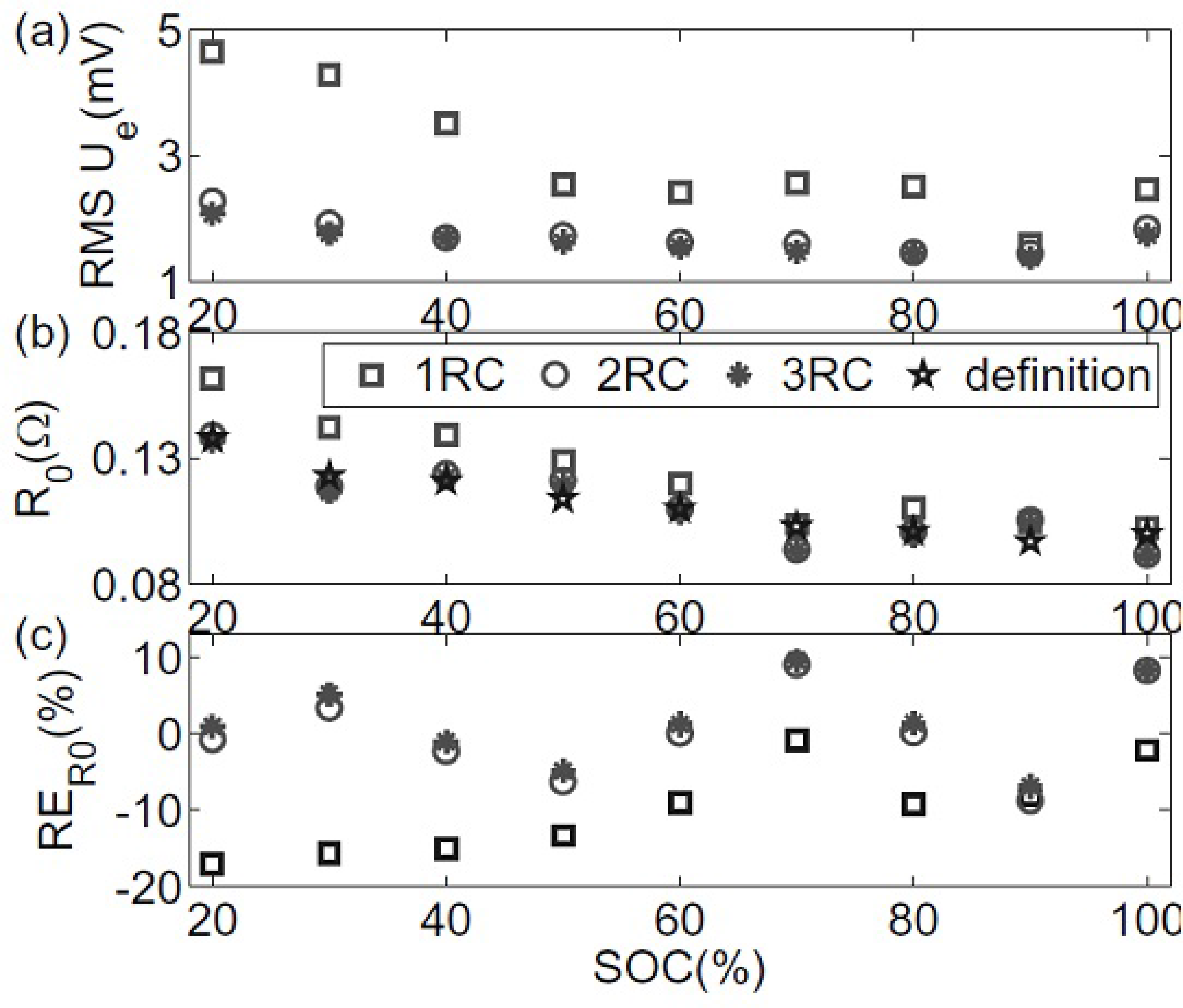
The root-mean-square (RMS) values of errors between the battery voltage simulation and measurements were used to evaluate the circuit model performance. The measurement value of ohmic resistance R₀ in Figure 1 was determined by the internal resistance definition [10]. Figure 2 shows the relative error results of the battery voltage and R₀ when the batteries discharged by 0.5 C pulse current series in the relaxation test. In the illustration of the RMS values of the battery voltage errors in Figure 2a, the three-RC-pair circuit model has the best approximation to the voltage measurements, with the mean, maximum, and minimum values equal to 1.6 mV, 2.083 mV, and 1.3851 mV, respectively. The voltage-fitting errors in mean RMS were shrunk 6.25% by the three-RC-pair circuit model compared to the two-RC-pair circuit model, and 87.5% compared to the one-RC-pair circuit model. For the ohmic resistance in Figure 2b, the three-RC-pair circuit model yielded the estimation values closest to the measurement values, the relative errors of which had the smallest RMS value equal to 5.44%, decreasing by 0.19% and 5.98% compared to the two-RC-pair circuit model and one-RC-pair circuit model, respectively, as shown in Figure 2c.

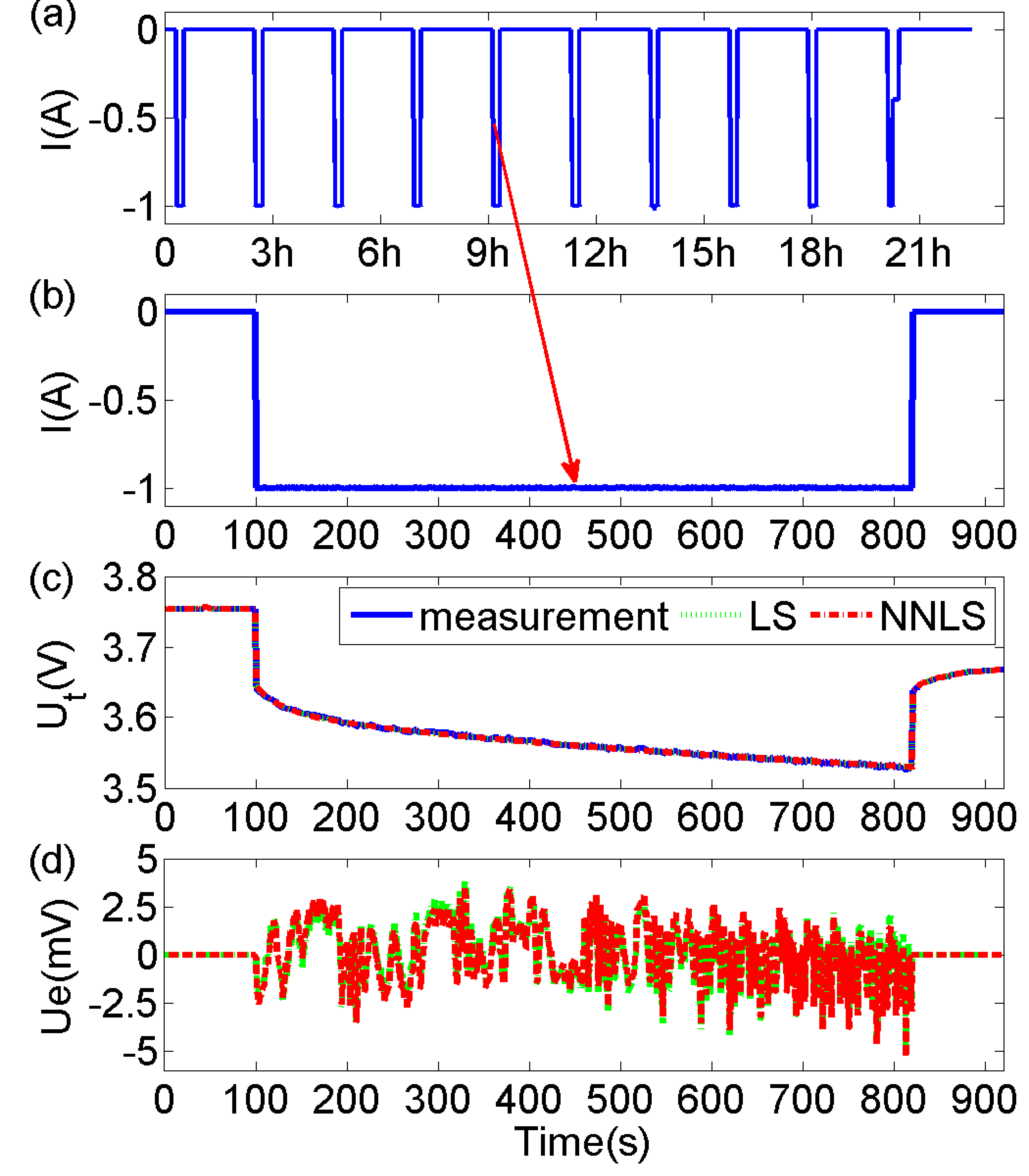
A three-RC-pair EEC in Figure 1 was used to model the Li-ion battery. One of the three-RC-pairs denoted the voltage drop caused by the combination of charge-transfer resistance and double-layer capacitance, one denoted the voltage drop generated by the Li-ion concentration gradient inside the battery, and one denoted the voltage drop resulting from the SEI layer growth. Moreover, the voltage fitting and ohmic estimation of the three-RC-pair circuit model was more accurate than the two-RC-pair and one-RC-pair circuit models. Additionally, when the number of RC pairs was more than 3 in the battery circuit model, the model generated a heavy computation load, the order of which could be reduced to that of the three-RC-pair circuit model by the NNLS algorithm. The parameters of the three-RC-pair circuit model were identified by the developed algorithm and normal LS. The measured and simulated results were exemplified at the battery SOC interval from 60% to 50% as shown in Figure 3. The corresponding model parameters and the RMS of the voltage errors are shown in

Table 4. Model parameters from SOC = 60% to 50% by 0.5 C pulse current discharge.

Method	LS		NNLS
Items	Resistance (Ω)	Capacitance (F)	Resistance (Ω)	Capacitance (F)
R0	0.10849	-	0.10861	-
RC1	0.03393	796	0.02363	889
RC2	0.02553	7,834	0.02586	3364
RC3	−0.01398	−64,378	0.00557	269,300
RMS (mV)	1.6		1.6

. Clearly, the positive parameters of the circuit model were estimated by the NNLS algorithm. However, there was one negative parameter equal to −13.98 mΩ estimated by the normal LS method, although the time constant of the one-RC pair was positive. Both of the voltage-error curves wavered within ±5 mV and had the same RMS value equal to 1.6 mV. The negative parameter of the one-RC pair means it always generates energy, which is not identical to the power consumption phenomena of a normal resistor. Moreover, there is no other energy-generation element inside the Li-ion battery except the electromotive force. By the comparable results, the positive parameter circuit model not only had the same voltage-fitting accuracy as the negative parameter circuit model, but represented the polarization effects on the voltage drop of the Li-ion battery.

4.2. Model Parameterization

Both look-up tables and equations were used to parameterize the three-RC-pair circuit model of the Li-ion battery because the OCV, resistance, and capacitance evolved with the working conditions. Assuming that the performance of the tested Li-ion battery would be hardly degraded at room temperature during the 2-week testing period, the model parameters would be minimally affected by the test time. At room temperature, the battery OCV was a function of the SOC, and the resistance and capacitance were functions of both the SOC and C-rate when the Li-battery worked.

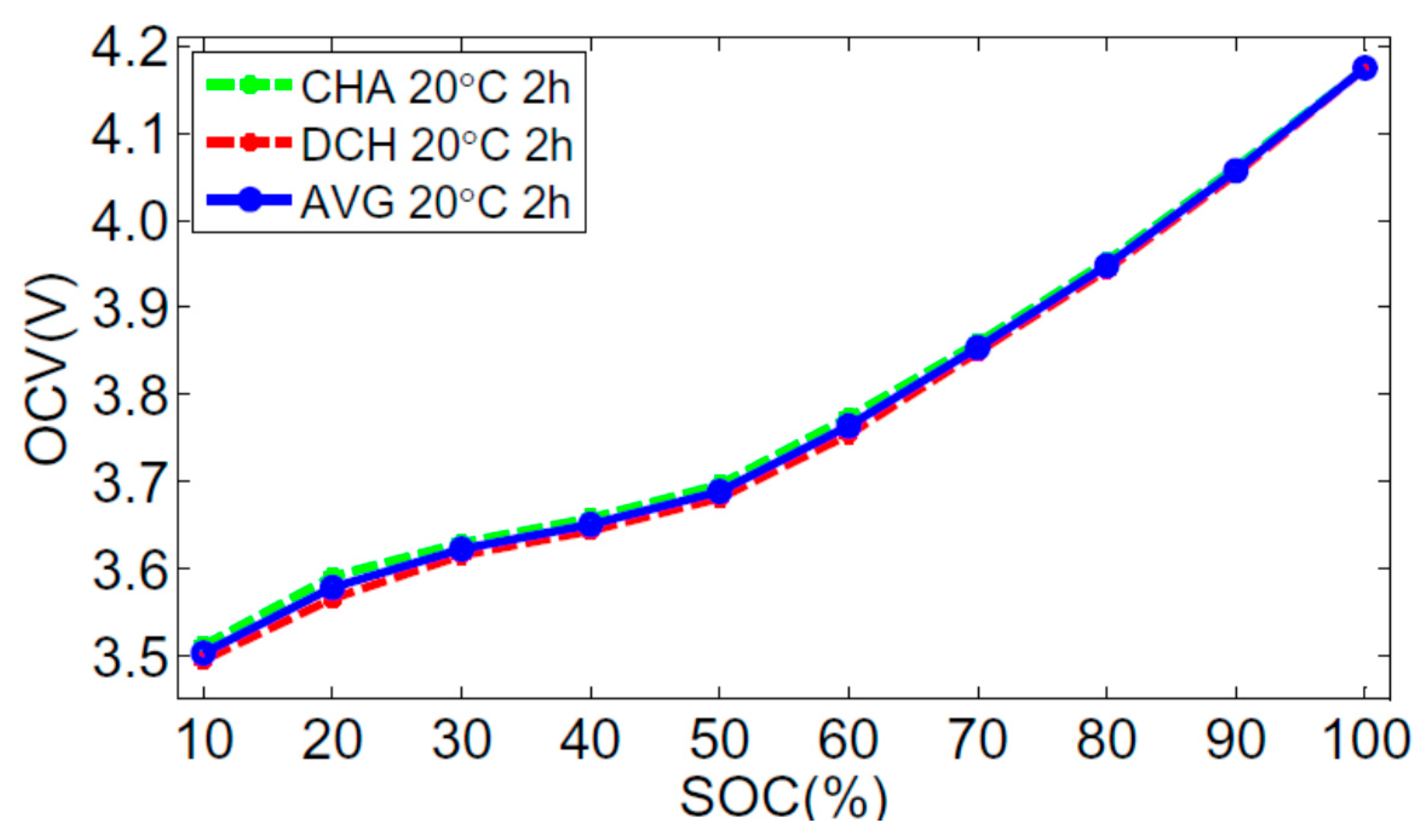
Figure 4 shows three SOC-OCV curves for battery discharging and charging, and their averaging. The absolute maximum, mean, and RMS of the relative errors of the hysteresis voltage between either discharging or charging and averaging OCVs at SOC points were about 0.35%, 0.18%, and 0.2%, respectively. The hysteresis voltage was so minimal that it could be neglected. The average of the charging and discharge curves could be used to establish the SOC-OCV relationship for Li-ion battery modeling.

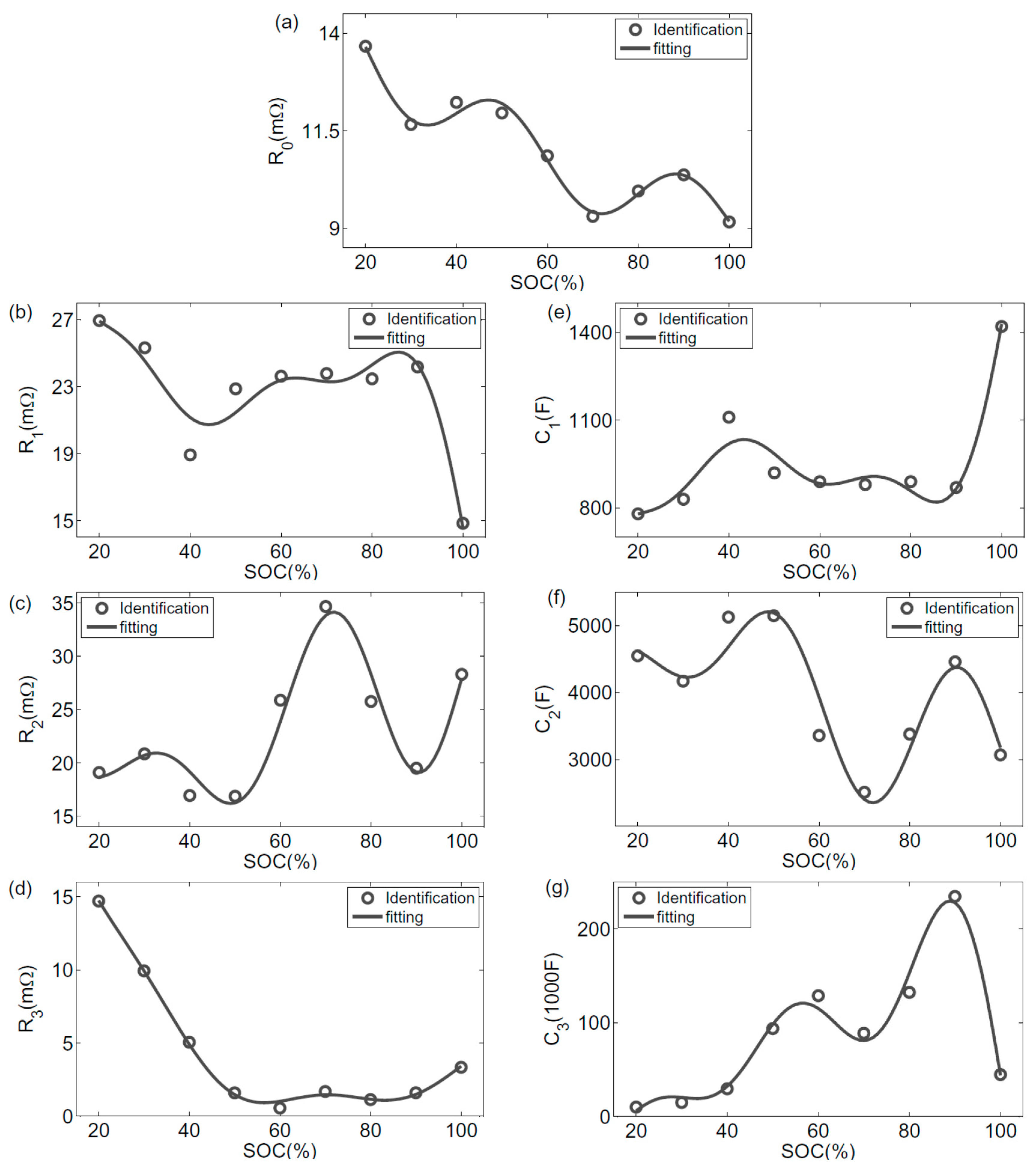
For the parameterization of the model resistance and capacitance, Equation (12) describes the relationships between each model parameter and the working conditions, including the SOC and C-rate. The trigonometric function polynomial (TFP) of Equation (11) is the parametric equation that depicts the changes of each model parameter with a single working condition. After the model parameters were extracted from the experiment data by the developed NNLS algorithm, the battery model was parameterized by the trigonometric function polynomials. The coefficients of Equation (11) for each model parameter were figured out at ω = 5π, N = 1, and M = 3 and are shown in

Table 5. Parametric equation coefficients of the solid lines in Figure 5.

Subplots	c0	c1	c2	c3	d0	d1
Figure 5a	0.1603	−0.1385	0.1054	−0.0354	0.0099	−0.0016
Figure 5b	0.0500	−0.1743	0.3331	−0.1942	−0.0046	0.0084
Figure 5c	0.0269	−0.0704	0.1653	−0.0939	0.0010	−0.0120
Figure 5d	0.3244	−1.1129	1.2210	−0.3984	−0.0113	0.0053
Figure 5e	−0.0323	0.8472	−1.6841	1.0121	0.0254	−0.0475
Figure 5f	0.2937	1.3824	−3.0339	1.6757	0.0182	0.1302
Figure 5g	0.1389	−1.2301	3.2583	−2.1232	−0.0746	0.1994

. The relationships between each model parameter and the battery SOC are illustrated at 0.5 C in Figure 5. The small circles denote the identified parameters of the three-RC-pair circuit model, and the solid lines show the fitting curves.

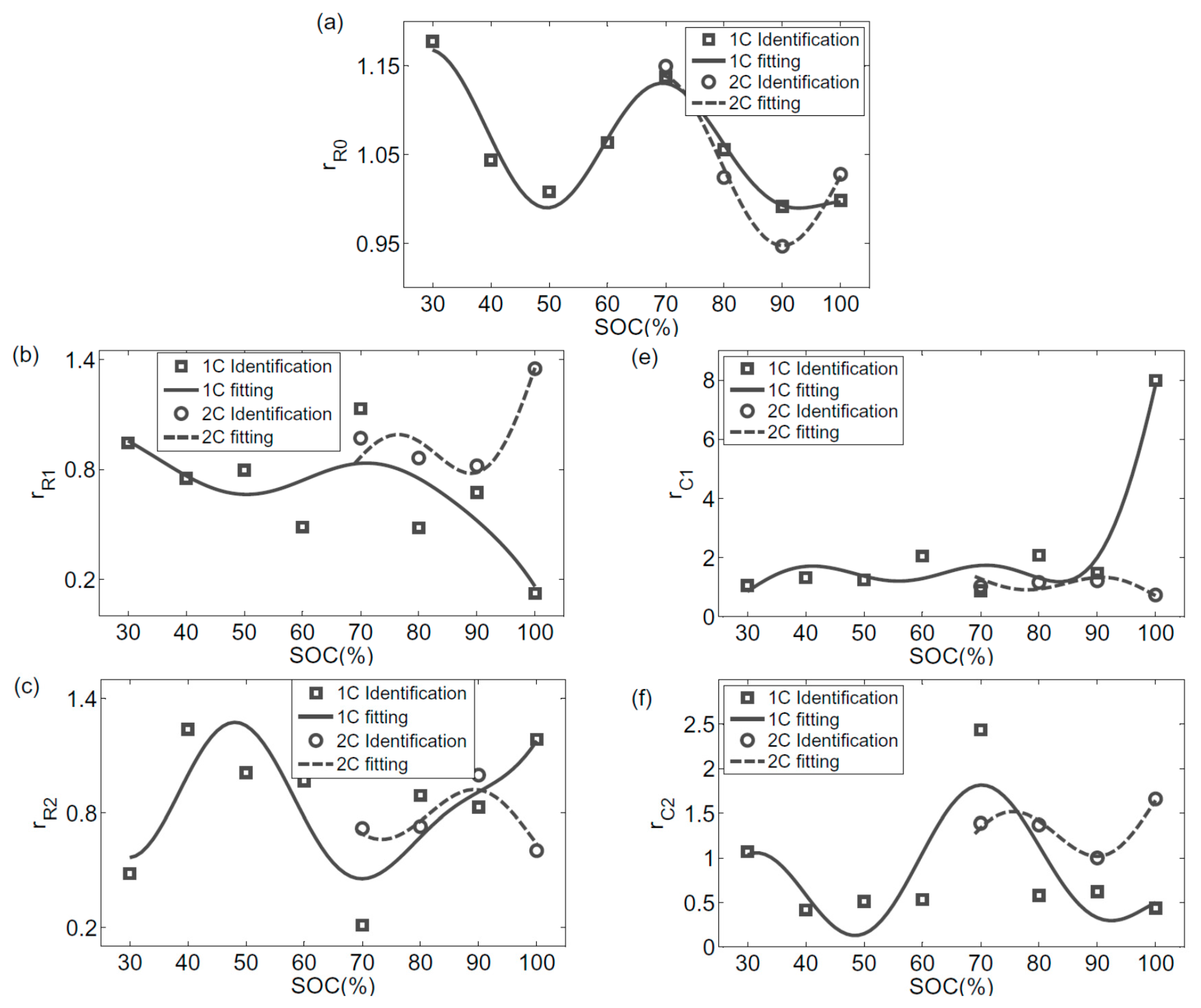
For the current-dependency model parameters, the amplitudes of pulse discharging C-rates stayed at 0.5 C, 1.0 C, and 2.0 C, respectively. A parameter ratio is defined as follows.

$$r=P_a/P_{0.5\mathrm{C}}$$

(13)

where P_a denotes each parameter extracted at any arbitrary C-rate discharge, and P_0.5C denotes each parameter extracted at 0.5 C discharge.

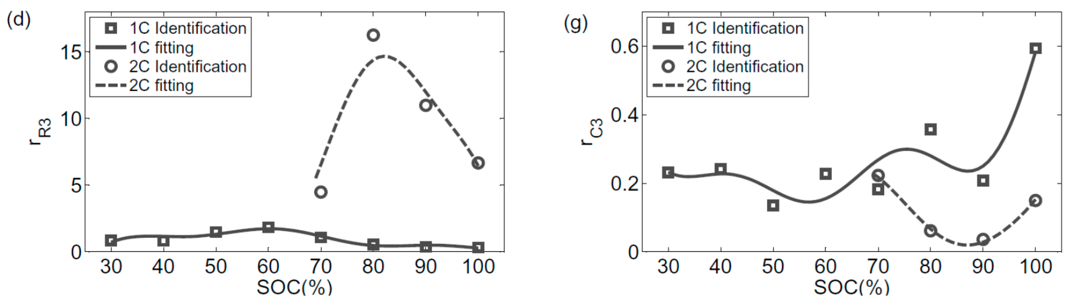
Each defined parameter ratio can also be used to build relationships with the C-rate by Equation (11). The model parameters at 1 C and 2 C are shown in Figure 6, the parametric equation of which has ω = 5π, N = 1, M = 4, and c₂ = 0 in Equation (11). The related coefficients of the parametric equations are presented in

Table 6. Parametric equation coefficients of the solid lines in Figure 6.

Subplots	c0	c1	c3	c4	d0	d1
Figure 6a	1.1400	−0.2629	0.8098	−0.6899	−0.1120	0.0710
Figure 6b	1.8279	−3.8193	10.7152	−8.5614	−0.0511	−0.0135
Figure 6c	0.9740	0.7140	−6.4647	5.9552	0.6933	−0.6603
Figure 6d	−8.1586	31.4145	−69.2239	46.2590	−1.6753	2.4123
Figure 6e	−5.4683	27.7815	−92.9621	78.4938	0.8357	−2.3330
Figure 6f	−0.6683	3.1911	0.8038	−2.8259	−0.8203	0.2380
Figure 6g	0.8209	−1.8465	2.7060	−1.0965	0.2285	−0.4339

for the solid lines in Figure 6 and

Table 7. Parametric equation coefficients of the dashed lines in Figure 6.

Subplots	c0	c1	c3	c4	d0	d1
Figure 6a	0.9336	0.5125	−1.3411	0.9210	−0.1231	0.0545
Figure 6b	3.7143	−9.4144	18.3809	−11.3248	0.7772	−1.3382
Figure 6c	−0.6789	5.4403	−11.9799	7.8573	−0.0141	0.3290
Figure 6d	86.1338	−302.9734	773.2776	−549.9901	18.2564	−25.1073
Figure 6e	−6.3770	−1.8927	−53.6968	35.4070	−1.8927	2.9712
Figure 6f	5.0609	−15.3247	36.4795	−24.5716	0.7567	−1.6425
Figure 6g	−0.8602	3.7671	−9.3643	6.6106	−0.2510	0.2650

for the dashed lines in Figure 6.

4.3. Model Verification

The developed parametric circuit modeling methodology was validated for the Li-ion battery by a random test profile. Meanwhile, both the lookup table and trigonometric function polynomial were applied to parameterize the proposed battery circuit model at room temperature.

A typical DST driving cycle is shown in Figure 7a. In order to verify the model robustness, a high current rate was used to charge/discharge the battery samples. The current amplitude of this profile was enlarged up to 4 A for battery discharging and 2 A for charging. The current profile was repeatedly applied to the battery cells from the full charge state to 20% SOC as shown in Figure 7b. The voltage differences equaled voltage measurements minus simulated values, and the relative errors of battery voltage are defined as the percent of ratio between voltage differences and measurements as follows:

$${\mathsf{\mu }}_c=100\%\times \left(u_t-u_t^{*}\right)/u_t$$

(14)

where u_t^* is the estimated voltage, and µ is the relative voltage error.

Impacted by the high discharging/charging current and compared to the real voltage as shown in Figure 7c, the two parameterization for the battery EEC model yielded voltage errors that stayed between –1% and 1% as shown in Figure 7d; the blue line denotes the model parameterization of the trigonometric function polynomial fitting, and the red line denotes the model parameterization of the lookup table. The RMS value of the voltage errors was 5.4 mV for the model parameterization of the lookup table, and decreased by 18% compared to that of the trigonometric function polynomial fitting. After 8100 s, the discharging/charging current amplitudes were reduced by 50%. Then the relative errors of the battery voltage shrunk. For example, the RMS value of the relative errors of the battery voltage between 8100 s and 16,001s was 0.16%, which was 0.04% less than that between 0 s and 8100 s shown by the blue line. The time scale was reduced from hours to seconds to check the voltages and their errors clearly. In the right-hand plots of Figure 7, the enlarged scope aimed at the maximum absolute value of relative errors is shown by green arrows and asterisks. The associated subplots are shown in Figure 7e–g. The voltage relative errors produced by the two battery models in Figure 7g showed similar tendencies. When the battery was discharged at 4 A, the battery models had the highest relative error points at 0.99% in the blue line and 0.84% in the red line, respectively. When the battery was charged at 2 A, the battery models had the lowest relative error points at −0.90% in the blue line and −0.71% in the red line, respectively. When the battery current varied between −1 A and 1 A, the voltage relative errors were less than 0.5%.

This new parameterization method used the current pulse series to extract positive parameters of the three-RC-pair EEC model for the Li-ion battery. The trigonometric function polynomial fitting technique for the battery circuit model resulted in similar voltage approximation accuracy as the lookup table.

5. Conclusions

A parametric circuit model for Li-ion batteries was developed and validated for applications such as electric vehicles. For this methodology, continuous-time circuit equations were developed to construct normal equations of both least squares and non-negative least squares to eliminate linear dependence between two columns of the related data matrix based on an easy equal-amplitude current pulse series. The non-negative least-squares method was first exploited to identify parameters of the equivalent circuit models of the Li-ion battery for positive values. Moreover, the combination of both non-negative least-squares and genetic algorithm was applied to estimate parameters of a three-RC-pair circuit model of the Li-ion battery, which was implemented by Matlab/Simulink^® software functions. Considering the effects of state-of-charge and C-rate on model parameters, a unified trigonometric function polynomial was developed to parameterize the battery circuit model compared to the commonly used lookup table for effectiveness and reliability. By using a random driving cycle, the voltage simulation accuracy of this parameterized model was validated. During the overall discharging cycle, the error between measured and simulated voltage stayed below 1%. This work contributes to developing a novel and reliable modeling methodology of Li-ion batteries for engineering applications based on the commonly used equal-amplitude pulse series of the battery current.

References

- Horiba, T. Lithium-ion battery systems. Proc. IEEE 2014, 102, 939–950. [Google Scholar] [CrossRef]
- Seaman, A.; Dao, T.S.; McPhee, J. A survey of mathematics-based equivalent-circuit and electrochemical battery models for hybrid and electric vehicle simulation. J. Power Sources 2014, 256, 410–423. [Google Scholar] [CrossRef]
- Stern, M.; Geary, A.L. Electrochemical polarization I. A theoretical analysis of the shape of polarization curves. J. Electrochem. Soc. 1957, 104, 56–63. [Google Scholar] [CrossRef]
- Paled, E. The electrochemical behavior of alkaliand alkaline earth metals in non-aqueous battery systems: The solid electrolyte interphase model. J. Electrochem. Soc. 1979, 126, 2047–2051. [Google Scholar] [CrossRef]
- Jeong, S.K.; Inaba, M.; Abe, T.; Ogumi, Z. Surface film formation on graphite negative electrodein lithium-ion batteries: AFM study in an ethylene carbonate-based solution. J. Electrochem. Soc. 2001, 148, 989–993. [Google Scholar] [CrossRef]
- Peled, E.; Golodnitsky, D.; Ardel, G. Advanced model for solid electrolyte interphase electrodes in liquid and polymer electrolytes. J. Electrochem. Soc. 1997, 144, 208–210. [Google Scholar] [CrossRef]
- Osaka, T.; Mukoyama, D.; Nara, H. Review—Development of diagnostic process for commercially available batteries, especially lithium ion battery by electrochemical impedance spectroscopy. J. Electrochem. Soc. 2015, 162, 2529–2537. [Google Scholar] [CrossRef]
- Lin, X.F.; Perez, H.E.; Mohan, S.; Siege, J.B.; Stefanopoulou, A.G.; Ding, Y.; Castanier, M.P. A lumped-parameter electro-thermal model for cylindrical batteries. J. Power Sources 2014, 257, 1–11. [Google Scholar] [CrossRef]
- Xia, B.; Wang, H.; Tian, Y.; Wang, M.; Sun, W.; Xu, Z. State of charge estimation of lithium-ion batteries using an adaptive cubature Kalman filter. Energies 2015, 8, 5916–5936. [Google Scholar] [CrossRef]
- Fleischer, C.; Waag, W.; Heyn, H.-M.; Sauer, D.U. On-line adaptive battery impedance parameter and state estimation considering physical principles in reduced order equivalent circuit battery models: Part 2. Parameter and state estimation. J. Power Sources 2014, 262, 457–482. [Google Scholar] [CrossRef]
- Feng, T.; Yang, L.; Zhao, X.; Zhang, H.; Qiang, J. Online identification of lithium-ion battery parameters based on an improved equivalent-circuit model and its implementation on battery state-of-power prediction. J. Power Sources 2015, 81, 192–203. [Google Scholar] [CrossRef]
- Mastali, M.; Vazquez-Arenas, J.; Fraser, R.; Fowler, M.; Afshar, S.; Stevens, M. Battery state of the charge estimation using Kalman filter. J. Power Sources 2013, 239, 294–307. [Google Scholar] [CrossRef]
- Xing, Y.; He, W.; Pecht, M.; Tsui, K.L. State of charge estimation of lithium-ion batteries using the open-circuit voltage at various ambient temperatures. Appl. Energy 2014, 113, 106–115. [Google Scholar] [CrossRef]
- Li, D.; Ouyang, J.; Li, H.; Wan, J. State of charge estimation for LiMn2O4 power battery based on strong tracking sigma point Kalman filter. J. Power Sources 2015, 279, 439–449. [Google Scholar] [CrossRef]
- Li, J.; Mazzola, M.S. Accurate battery pack modeling for automotive applications. J. Power Sources 2013, 237, 215–228. [Google Scholar] [CrossRef]
- Hua, X.S.; Li, S.B.; Peng, H. A comparative study of equivalent circuit models for Li-ion batteries. J. Power Sources 2012, 198, 359–367. [Google Scholar] [CrossRef]
- Jackey, R.; Saginaw, M.; Sanghvi, P.; Gazzarri, J.; Huria, T.; Ceraolo, M. Battery Model Parameter Estimation Using a Layered Technique: An Example Using a Lithium Iron Phosphate Cell. SAE Tech. Pap. 2013. [Google Scholar] [CrossRef]
- Huria, T.; Ludovici, G.; Lutzemberger, G. State of charge estimation of high power lithium iron phosphate cells. J. Power Sources 2014, 249, 92–102. [Google Scholar] [CrossRef]
- Einhorn, M.; Conte, F.V.; Kral, C.; Fleig, J. Comparison, selection, and parameterization of electrical battery models for automotive applications. IEEE Trans. Power Electron. 2013, 28, 1429–1437. [Google Scholar] [CrossRef]
- Andre, D.; Meiler, M.; Walz, K.S.H.; Soczka-Guth, T.; Sauer, D.U. Characterization of high-power lithium-ion batteries by electrochemical impedance spectroscopy. II: Modelling. J. Power Sources 2011, 196, 5349–5356. [Google Scholar] [CrossRef]
- Aung, H.; Low, K.S.; Goh, S.T. State-of-charge estimation of lithium-ion battery using square root spherical unscented Kalman filter (Sqrt-UKFST) in nanosatellite. IEEE Trans. Power Electron. 2015, 30, 4774–4783. [Google Scholar] [CrossRef]
- Dubarry, M.; Liaw, B.Y. Development of a universal modeling tool for rechargeable lithium batteries. J. Power Sources 2007, 174, 856–860. [Google Scholar] [CrossRef]
- Lawson, C.L.; Hanson, R.J. Solving Least Squares Problems; Prentice Hall: Upper Saddle River, NJ, USA, 1974. [Google Scholar]
- Waag, W.; Fleischer, C.; Sauer, D.U. Critical review of the methods for monitoring of lithium-ion batteries in electric and hybrid vehicles. J. Power Sources 2014, 258, 321–339. [Google Scholar] [CrossRef]
Figure 1.
Equivalent circuit model for a Li-ion battery.
Figure 2.
The model performance evaluation: (a) voltage error in RMS, RMS Ue; (b) ohmic resistance, R0; (c) relative errors of R0, .
Figure 3.
Battery voltage and voltage errors of the three-RC-pair circuit model from SOC = 60% to 50%: (a) a current pulse series: the unit for the x-axis is hours; (b) current; (c) voltage; (d) voltage error.
Figure 4.
Battery SOC-OCV curves: CHA, charging; DCH, discharging; AVG, averaging.
Figure 5.
Battery model parameters at 0.5C: (a) internal resistance, R0; (b) polarization resistance, R1; (c) polarization resistance, R2; (d) polarization resistance, R3; (e) polarization capacitance, C1; (f) polarization capacitance, C2; (g) polarization capacitance, C3.
Figure 6.
Battery model parameter ratios at 1 C and 2 C: (a) internal resistance ratio, rR0; (b) polarization resistance ratio, rR1; (c) polarization resistance ratio, rR2; (d) polarization resistance ratio, rR3; (e) polarization capacitance ratio, rC1; (f) polarization capacitance ratio, rC2; (g) polarization capacitance ratio, rC3.
Figure 7.
Battery model validation profiles: (a) current, I; (b) SOC; (c) voltage, ut; (d) voltage relative errors, µc; (e) enlarged current, I; (f) enlarged voltage, ut; (g) enlarged voltage relative errors, µc. ** Note: in the left-hand subplot (d). This data window started from 7300 s, the 180 s duration of which was enlarged for the right-hand subplots (e–g).