


ABSTRACT
We perform a Bayesian analysis of the mass distribution of stellar-mass black holes using the observed masses of 15 low-mass X-ray binary systems undergoing Roche lobe overflow and 5 high-mass, wind-fed X-ray binary systems. Using Markov Chain Monte Carlo calculations, we model the mass distribution both parametrically—as a power law, exponential, Gaussian, combination of two Gaussians, or log-normal distribution—and non-parametrically—as histograms with varying numbers of bins. We provide confidence bounds on the shape of the mass distribution in the context of each model and compare the models with each other by calculating their relative Bayesian evidence as supported by the measurements, taking into account the number of degrees of freedom of each model. The mass distribution of the low-mass systems is best fit by a power law, while the distribution of the combined sample is best fit by the exponential model. This difference indicates that the low-mass subsample is not consistent with being drawn from the distribution of the combined population. We examine the existence of a "gap" between the most massive neutron stars and the least massive black holes by considering the value, M1%, of the 1% quantile from each black hole mass distribution as the lower bound of black hole masses. Our analysis generates posterior distributions for M1%; the best model (the power law) fitted to the low-mass systems has a distribution of lower bounds with M1%>4.3 M☉ with 90% confidence, while the best model (the exponential) fitted to all 20 systems has M1%>4.5 M☉ with 90% confidence. We conclude that our sample of black hole masses provides strong evidence of a gap between the maximum neutron star mass and the lower bound on black hole masses. Our results on the low-mass sample are in qualitative agreement with those of Ozel et al., although our broad model selection analysis more reliably reveals the best-fit quantitative description of the underlying mass distribution. The results on the combined sample of low- and high-mass systems are in qualitative agreement with Fryer & Kalogera, although the presence of a mass gap remains theoretically unexplained.
Export citation and abstract BibTeX RIS
1. INTRODUCTION
The most massive stars probably end their lives with a supernova explosion or a quiet core collapse, becoming stellar-mass black holes. The mass distribution of such black holes can provide important clues to the end stages of evolution of these stars. In addition, the mass distribution of stellar-mass black holes is an important input in calculations of rates of gravitational wave emission events from coalescing neutron star–black hole and black hole–black hole binaries in the LIGO gravitational wave observatory (Abadie et al. 2010).
Observations of X-ray binaries in both the optical and X-ray bands can provide a measurement of the mass of the compact object in these systems. The current sample of stellar-mass black holes with dynamically measured masses includes 15 systems with low-mass, Roche lobe overflowing donors and 5 wind-fed systems with high-mass donors. Hence, sophisticated statistical analyses of the black hole mass distribution in these systems are possible.
The first study of the mass distribution of stellar-mass black holes, in Bailyn et al. (1998), examined a sample of seven low-mass X-ray binaries thought to contain a black hole, concluding in a Bayesian analysis that the mass function was strongly peaked around seven solar masses.5 Bailyn et al. (1998) found evidence of a "gap" between the least massive black hole and a "safe" upper limit for neutron star masses of 3 M☉ (e.g., Kalogera & Baym 1996). Such a gap is puzzling in light of theoretical studies that predict a continuous distribution of compact object supernova remnant masses with a smooth transition from neutron stars to black holes (Fryer & Kalogera 2001). (We note that Fryer & Kalogera (2001) considered binary evolution effects only heuristically and put forward some possible explanations for the gap from Bailyn et al. (1998) both in the context of selection effects or in connection to the energetics of supernova explosions.)
Toward the end of our analysis work, we became aware of a more recent study (Ozel et al. 2010), also in a Bayesian framework, analyzing the low-mass X-ray binary sample. Our results are largely consistent with those obtained by Ozel et al. (2010), who examined 16 low-mass X-ray binary systems containing black holes and found a strongly peaked distribution at 7.8 ± 1.2 M☉. They used two models for the mass function: a Gaussian and a decaying exponential with a minimum "turn-on" mass (motivated by the analytical model of the black hole mass function in Fryer & Kalogera 2001). We note that Ozel et al. (2010) do not provide confidence limits for the minimum black hole mass, instead discussing only the model parameters at the peak of their posterior distributions. They also do not perform any model selection analysis; thus, they give the distribution of parameters within each of their models, but cannot say which model is more likely to correspond to the true distribution of black hole masses. Nevertheless, it appears that their analysis confirms the existence of a mass gap. Ozel et al. (2010) discuss possible selection effects that could lead to the appearance of a mass gap, but conclude that these effects could not produce the observed gap, which they therefore claim is a real property of the black hole mass distribution.
We use a Bayesian Markov Chain Monte Carlo (MCMC) analysis to quantitatively assess a wide range of models for the black hole mass function for both samples. We include both parametric models, such as a Gaussian, and non-parametric models where the mass function is represented by histograms with various numbers of bins. (Our set of models includes those of Ozel et al. 2010 and Bailyn et al. 1998.) After computing posterior distributions for the model parameters, we use model selection techniques (including a new technique for efficient reversible-jump MCMC; Farr & Mandel 2011) to compare the evidence for the various models from both samples.
We define the "minimum black hole mass" to be the 1% quantile,  , in the black hole mass distribution (see Section 5). In qualitative agreement with Ozel et al. (2010) and Bailyn et al. (1998), we find strong evidence for a mass gap among the best models for both samples. Our analysis gives distributions for
  implied by the data in the context of each of our models for the black hole mass distribution. In the context of the best model for the low-mass systems (a power law), the distribution for
  gives
gives  with 90% confidence; in the context of the best model for the combined sample of lower- and high-mass systems the distribution of
  has
has  with 90% confidence. Further, in the context of models with lower evidence, most also have a mass gap, with 90% confidence bounds on
  significantly above a "safe" maximum neutron star mass of 3 M☉ (Kalogera & Baym 1996).
We find that, for the low-mass X-ray binary sample, the theoretical model from Fryer & Kalogera (2001)—a decaying exponential—is strongly disfavored by our model selection. We find that the low-mass systems are best described by a power law, followed closely by a Gaussian (which is the second model considered by Ozel et al. 2010). On the other hand, we find that the theoretical model from Fryer & Kalogera (2001) is the preferred model for the combined sample of low- and high-mass X-ray binaries. A model with two separate Gaussian peaks also has relatively high evidence for the combined sample of systems. The difference in best-fitting model indicates that the low-mass subsample is not consistent with being drawn from the distribution of the combined population.
The structure of this paper is as follows. In Section 2, we discuss the 15 systems that comprise the low-mass X-ray binary black hole sample and the 5 additional high-mass, wind-fed systems that make up the combined sample. In Section 3, we discuss the Bayesian techniques we use to analyze the black hole mass distribution, the techniques we use for model selection, and the parametric and non-parametric models we will use for the black hole mass distribution. In Section 4, we discuss the results of our analysis and model selection. In Section 5, we discuss the distribution of the minimum black hole mass implied by the analysis of Section 4. In Section 6, we summarize our results and comment on the significance of the observed mass gap in the context of theoretical models. Appendix A describes MCMC techniques in some detail. Appendix B explains our novel algorithm for efficiently performing the reversible-jump MCMC computations used in the model comparisons of Section 4 (but see also Farr & Mandel 2011).
2. SYSTEMS
The 20 X-ray binary systems on which this study is based are listed in Table 1. We separate the systems into 15 low-mass systems in which the central black hole appears to be fed by Roche lobe overflow from the secondary, and 5 high-mass systems in which the black hole is fed via winds (these systems all have a secondary that appears to be more massive than the black hole). The low- and high-mass systems undoubtedly have different evolutionary tracks, and therefore it is reasonable that they would have different black hole mass distributions. We will first analyze the 15 low-mass systems alone (Section 4.1), and then the combined sample of 20 systems (Section 4.2).
Table 1. The Source Parameters for the 20 X-ray Binaries Used in This Work
| Source | f (M☉) | q | i (deg) | References |
|---|---|---|---|---|
| GRS 1915 | N(9.5, 3.0) | N(0.0857, 0.0284) | N(70, 2) | Greiner et al. (2001) |
| XTE J1118 | N(6.44, 0.08) | N(0.0264, 0.004) | N(68, 2) | Gelino et al. (2008) |
| Harlaftis & Filippenko (2005) | ||||
| XTE J1650 | N(2.73, 0.56) | U(0, 0.5) | I(50, 80) | Orosz et al. (2004) |
| GRS 1009 | N(3.17, 0.12) | N(0.137, 0.015) | I(37, 80) | Filippenko et al. (1999) |
| A0620 | N(2.76, 0.036) | N(0.06, 0.004) | N(50.98, 0.87) | Cantrell et al. (2010) |
| Neilsen et al. (2008) | ||||
| GRO J0422 | N(1.13, 0.09) | U(0.076, 0.31) | N(45, 2) | Gelino & Harrison (2003) |
| Nova Mus 1991 | N(3.01, 0.15) | N(0.128, 0.04) | N(54, 1.5) | Gelino et al. (2001) |
| GRO J1655 | N(2.73, 0.09) | N(0.3663, 0.04025) | N(70.2, 1.9) | Greene et al. (2001) |
| 4U 1543 | N(0.25, 0.01) | U(0.25, 0.31) | N(20.7, 1.5) | Orosz (2003) |
| XTE J1550 | N(7.73, 0.4) | U(0, 0.04) | N(74.7, 3.8) | Orosz et al. (2011) |
| V4641 Sgr | N(3.13, 0.13) | U(0.42, 0.45) | N(75, 2) | Orosz (2003) |
| GS 2023 | N(6.08, 0.06) | U(0.056, 0.063) | I(66, 70) | Charles & Coe (2006) |
| Khargharia et al. (2010) | ||||
| GS 1354 | N(5.73, 0.29) | N(0.12, 0.04) | I(50, 80) | Casares et al. (2009) |
| Nova Oph 77 | N(4.86, 0.13) | U(0, 0.053) | I(60, 80) | Charles & Coe (2006) |
| GS 2000 | N(5.01, 0.12) | U(0.035, 0.053) | I(43, 74) | Charles & Coe (2006) |
| Cyg X1 | N(0.251, 0.007) | N(2.778, 0.386) | I(23, 38) | Gies et al. (2003) |
| M33 X7 | N(0.46, 0.08) | N(4.47, 0.61) | N(74.6, 1) | Orosz et al. (2007) |
| NGC 300 X1 | N(2.6, 0.3) | U(1.05, 1.65) | I(60, 75) | Crowther et al. (2010) |
| LMC X1 | N(0.148, 0.004) | N(2.91, 0.49) | N(36.38, 2.02) | Orosz et al. (2009) |
| IC 10 X1 | N(7.64, 1.26) | U(0.7, 1.7) | I(75, 90) | Prestwich et al. (2007) |
| Silverman & Filippenko (2008) | ||||
Notes. The first 15 systems have low-mass secondaries that feed the black hole via Roche lobe overflow; the last 5 systems have high-mass secondaries (q ≳ 1) that feed the black hole via winds. In each line, f is the mass function for the compact object, q is the mass ratio M2/M, and i is the inclination of the system to the line of sight. We indicate the distribution used for the true parameters when computing the probability distributions for the masses of these systems: N(μ, σ) implies a Gaussian with mean μ and standard deviation σ, U(a,b) is a uniform distribution between a and b, and I(α, β) is an isotropic distribution between the angles α and β.
Download table as: ASCIITypeset image
In each of these systems, spectroscopic measurements of the secondary star provide an orbital period for the system and a semi-amplitude for the secondary's velocity curve. These measurements can be combined into the mass function,
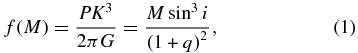
where P is the orbital period, K is the secondary's velocity semi-amplitude, M is the black hole mass, i is the inclination of the system, and q ≡ M2/M is the mass ratio of the system.
The mass function defines a lower limit on the mass: f(M) < M. To accurately determine the mass of the black hole, the inclination i and mass ratio q must be measured. Ideally, this can be accomplished by fitting ellipsoidal light curves and study of the rotational broadening of spectral lines from the secondary, but even in the most studied case (see, e.g., Cantrell et al. 2010 on A0620) this procedure is complicated. In particular, contributions from an accretion disk and hot spots in the disk can significantly distort the measured inclination and mass ratios. For some systems (e.g., GS 1354; Casares et al. 2009) strong variability completely prevents determination of the inclination from the light curve; in these cases an upper limit on the inclination often comes from the observed lack of eclipses in the light curve. In general, accurately determining q and i requires a careful system-by-system analysis.
For the purposes of this paper, we adopt the following simplified approach to the estimation of the black hole mass from the observed data. When an observable is well constrained, we assume that the true value is normally distributed about the measured value with a standard deviation equal to the quoted observational error. This is the case for the mass function in all the systems we use, and for many systems' mass ratios and inclinations. When a large range is quoted in the literature for an observable, we take the true value to be distributed uniformly (for the mass ratio) or isotropically (for the inclination) within the quoted range. Table 1 gives the assumed distribution for the observables in the 20 systems we use. We do not attempt to deal with the systematic biases in the observational determination of f, q, and i in any realistic way; we are currently investigating more realistic treatments of the errors (including observational biases that can shift the peak of the true mass distribution away from the "best-fit" mass in the observations). This treatment will appear in future work.
From these assumptions, we can generate probability distributions for the true mass of the black hole given the observations and errors via the Monte Carlo method: drawing samples of f, q, and i from the assumed distributions and computing the mass implied by Equation (1) gives samples of M from the distribution induced by the relationship in Equation (1). Mass distributions generated in this way for the systems used in this work are shown in Figures 1 and 2. Systems for which i is poorly constrained have broad "tails" on their mass distributions. These mass distributions constitute the "observational data" we will use in the remainder of this paper.
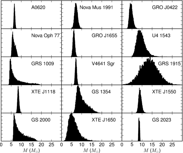
Figure 1. Individual mass distributions implied by Equation (1) and the assumed distributions on observational parameters f, q, and i given in Table 1 for the low-mass sources. The significant asymmetry and long tails in many of these distributions are the result of the nonlinear relationship (Equation (1)) between M, f, q, and i.
Download figure:
Standard image High-resolution image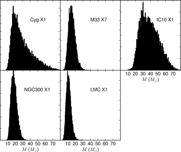
Figure 2. Mass distributions for the wind-fed, high-mass systems computed from the distributions on observed data in Table 1 using Equation (1). (Similar to Figure 1.) The asymmetry and long tails in these distributions are the result of the nonlinear relationship between M, f, q, and i.
Download figure:
Standard image High-resolution image3. STATISTICAL ANALYSIS
In this section, we describe the statistical analysis we will apply to various models for the underlying mass distribution from which the low-mass sample and the combined sample of X-ray binary systems in Table 1 were drawn. The results of our analysis are presented in Section 4.
3.1. Bayesian Inference
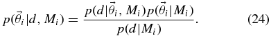
The end result of our statistical analysis will be the probability distribution for the parameters of each model implied by the data from Section 2 in combination with our prior assumptions about the probability distribution for the parameters. Bayes' rule relates these quantities. For a model with parameters  in the presence of data d, Bayes' rule states
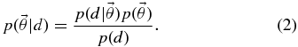
Here,  , called the posterior probability distribution function, is the probability distribution for the parameters
  implied by the data d;
  , called the likelihood, is the probability of observing data d given that the model parameters are
  ;
;  , called the prior, reflects our estimate of the probability of the various model parameters in the absence of any data; and p(d), called the evidence, is an overall normalizing constant ensuring that
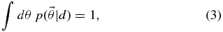
whence
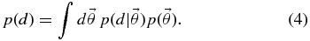
In our context, the data are the mass distributions given in Section 2: d = {pi(M)|i = 1, 2, ..., 20}. We assume that the measurements in Section 2 are independent, so the complete likelihood is given by a product of the likelihoods for the individual measurements. For a model with parameters  that predicts a mass distribution
  for black holes, we have
That is, the likelihood of an observation is the average over the individual mass distribution implied by the observation, pi(M), of the probability for a black hole of that mass to exist according to the model of the mass distribution,  . We approximate the integrals as averages of
  over the Monte Carlo mass samples drawn from the distributions in Table 1 (also see Figures 1 and 2):

where Mij is the jth sample (out of a total Ni) from the ith individual mass distribution.
Our calculation of the likelihood of each observation does not include any attempt to account for selection effects in the observations. We simply assume (almost certainly incorrectly) that any black hole drawn from the underlying mass distribution is equally likely to be observed. The results of Ozel et al. (2010) suggest that selection effects are unlikely to significantly bias our analysis.
For a mass distribution with several parameters,  lives in a multi-dimensional space. Previous works (Ozel et al. 2010; Bailyn et al. 1998) have considered models with only two parameters; for such models evaluating
  on a grid may be a reliable method. Many of our models for the underlying mass distribution have three or more parameters. Exploring the entirety of these parameter spaces with a grid rapidly becomes prohibitive as the number of parameters increases. A more efficient way to explore the distribution
  is to use a MCMC method (see Appendix A). MCMC methods produce a chain (sequence) of parameter samples,
  , such that a particular parameter sample,
  , appears in the sequence with a frequency proportional to its posterior probability,
  . In this way, regions of parameter space where
  is large are sampled densely while regions where
  is small are effectively ignored.
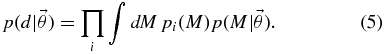
Once we have a chain of samples from  , the distribution for any quantity of interest can be computed by evaluating it on each sample in the chain and forming a histogram of these values. For example, to compute the one-dimensional distribution for a single parameter obtained by integrating over all other dimensions in parameter space, called the "marginalized" distribution, one plots the histogram of the values of that parameter appearing in the chain.
3.2. Priors
An important part of any Bayesian analysis is the priors placed on the parameters of the model. The choice of priors can bias the results of the analysis through both the shape and the range of prior support in parameter space. The prior should reflect the "best guess" for the distribution of parameters before examining any of the data. In the absence of any information about the distribution of parameters, it is best to choose a prior that is broad and uninformative to avoid biasing the posterior as much as possible.
A prior that is independent of parameters,  , in some region, called "flat," results in a posterior that is proportional to the likelihood (see Equation (2)). A flat prior does not change the shape of the posterior. However, the choice of a flat prior is parameterization dependent: a change of parameter from
  to
to  can change a flat distribution into one with non-trivial structure. In this work, we choose priors that are flat when the parameters are measured in physical units. In particular, for the log-normal model (Section 3.3.4) the natural parameters for the distribution are the mean, 〈log M〉, and standard deviation, σlog M, in log M, but we choose priors that are flat in 〈M〉 and σM.
The range of prior support can also affect the results of a Bayesian analysis. Because priors are normalized, prior support over a larger region of parameter space results in a smaller prior probability at each point. Such "wide" priors are implicitly claiming that any particular sub-region of parameter space is less likely than it would be under a prior of the same shape but smaller support volume. This difference is important in model selection (Section 3.5): when comparing two models with the same likelihood, one with wide priors will seem less probable than one with narrower priors. Of course, priors should be wide enough to encompass all regions of parameter space that have significant likelihood. To make the model comparison in Section 3.5 fair, we choose prior support in parameter space so that the allowed parameter values for each model give distributions for which nearly all the probability lies in the range 0 M☉ ⩽ M ⩽ 40 M☉.
3.3. Parametric Models for the Black Hole Mass Distribution
Here, we discuss the various parametric models of the underlying black hole mass distribution considered in this paper.
3.3.1. Power-law Models
Many astrophysical distributions are power laws. Let us assume that the black hole mass distribution is given by
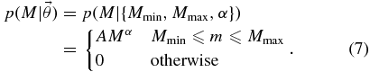
The normalizing constant A is
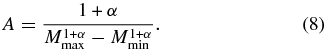
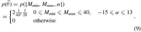
We choose uniform priors on Mmin and Mmax ⩾ Mmin between 0 and 40 M☉, and uniform priors on the exponent α in a broad range between −15 and 13:
Our MCMC analysis output is a list of {Mmin, Mmax, α} values distributed according to the posterior
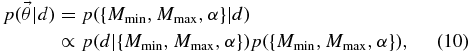
with the likelihood p(d|{Mmin, Mmax, α}) defined in Equation (5).
3.3.2. Decaying Exponential
Fryer & Kalogera (2001) studied the relation between progenitor and remnant mass in simulations of supernova explosions. Combining this with the mass function for supernova progenitors, they suggested that the black hole mass distribution may be well represented by a decaying exponential with a minimum mass:
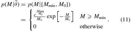
We choose a prior for this model where Mmin is uniform between 0 and 40 M☉. For each Mmin, we choose M0 uniformly within a range ensuring that 40 M☉ is at least two scale masses above the cutoff: 40 M☉ ⩾ Mmin + 2M0. This ensures that the majority of the mass probability lies in the range 0 M☉ ⩽ M ⩽ 40 M☉. The resulting prior is
3.3.3. Gaussian and Two-Gaussian Models
The mass distributions in Figure 1 all peak in a relatively narrow range near ∼10 M☉. The prototypical single-peaked probability distribution is a Gaussian:
We use a prior on the mean mass, μ, and the standard deviation, σ, that ensures that the majority of the mass distribution lies below 40 M☉:
where both μ and σ are measured in solar masses.
Though we do not expect to find a second peak in the low-mass distribution, we may find evidence of one when exploring the combined low- and high-mass samples. To look for a second peak in the black hole mass distribution, we use a two-Gaussian model:
The probability is a linear combination of two Gaussians with weights α and 1 − α. We restrict μ1 < μ2 and also impose combined conditions on μi and σi that ensure that most of the mass probability lies below 40 M☉ with the prior
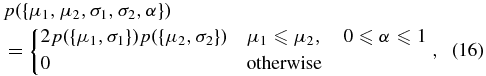
where the single-Gaussian prior, p({μi, σi}), is defined in Equation (14).
3.3.4. Log Normal
Many of the mass distributions for the systems in Figure 1 rise rapidly to a peak and then fall off more slowly in a longer tail toward high masses. So far, none of the parameterized distributions we have discussed have this property. In this section, we consider a log-normal model for the underlying mass distribution; the log-normal distribution has a rise to a peak with a slower falloff in a long tail.
The log-normal distribution gives log M a Gaussian distribution with mean μ and standard deviation σ:
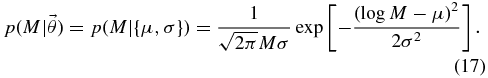
The parameters μ and σ are dimensionless; the mean mass 〈M〉 and mass standard deviation σM are related to μ and σ by
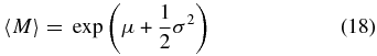
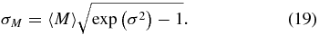
For a fair comparison with the other models, we impose a prior that is flat in 〈M〉 and σM. To ensure that most of the probability in this model occurs for masses below 40 M☉, we require 〈M〉 + 2σM ⩽ 40, resulting in a prior
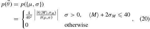
where
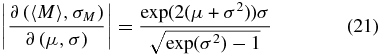
is the determinant of the Jacobian of the map in Equations (18) and (19).
3.4. Non-parametric Models for the Black Hole Mass Distribution
The previous subsection discussed models for the underlying black hole mass distribution that assumed particular parameterized shapes for the distribution. In this subsection, we will discuss models that do not assume a priori a shape for the black hole mass distribution. The fundamental non-parametric distribution in this section is a histogram with some number of bins, Nbin. Such a distribution is piecewise constant in M.
One choice for representing such a histogram would be to fix the bin locations, and allow the heights to vary. With this approach, one should be careful not to "split" features of the mass distribution across more than one bin in order to avoid diluting the sensitivity to such features; similarly, one should avoid including more than "one" feature in each bin. The locations of the bins, then, are crucial. An alternative representation of histogram mass distributions avoids this difficulty.
We choose to represent a histogram mass distribution with Nbin bins by allocating a fixed probability, 1/Nbin, to each bin. The lower and upper bounds for each bin are allowed to vary; when these are close to each other (i.e., the bin is narrow), the distribution will have a large value, and conversely when the bounds are far from each other. We assume that the non-zero region of the distribution is contiguous, so we can represent the boundaries of the bins as a non-decreasing array of masses,  , with w0 the minimum and
  the maximum mass for which the distribution has support. This gives the distribution
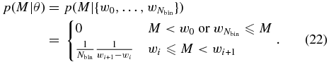
For priors on the histogram model with Nbin bins, we assume that the bin boundaries are uniformly distributed between 0 and 40 M☉ subject only to the constraint that the boundaries are non-decreasing from w0 to  :
:
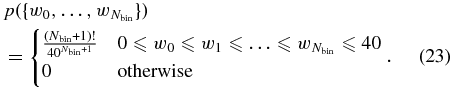
We consider histograms with up to five bins in this work. We will see that the evidence for the histogram models (see Sections 3.5, 4.1.7, and 4.2.7) from both the low-mass and combined data sets is decreasing as the number of bins reaches five, indicating that increasing the number of bins beyond five would not sufficiently improve the fit to the mass distribution to compensate for the extra parameter space volume implied by the additional parameters.
3.5. Bayesian Model Selection
In Sections 3.3 and 3.4, we discussed a series of models for the underlying black hole mass distribution. Our MCMC analysis will provide the posterior distribution of the parameters within each model, but does not tell us which models are more likely to correspond to the actual distribution. This model selection problem is the topic of this section.
Consider a set of models, {Mi|i = 1, ...}, each with corresponding parameters  . Re-writing Equation (2) to be explicit about the assumption of a particular model, we have
This gives the posterior probability of the parameters  in the context of model Mi. But the model itself can be regarded as a discrete parameter in a larger "super-model" that encompasses all the Mi. The parameters for the super-model are
  : a choice of model and the corresponding parameter values within that model. Each point in the super-model parameter space is a statement that, e.g., "the underlying mass distribution is a Gaussian, with parameters μ and σ," or "the underlying mass distribution is a triple-bin histogram with parameters w1, w2, w3, and w4," or... The posterior probability of the super-model parameters is given by Bayes' rule:
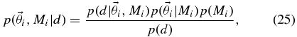
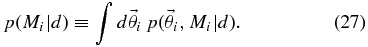
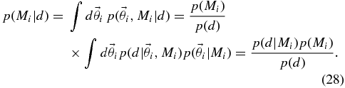
where we have introduced the model prior p(Mi), which represents our estimate on the probability that model Mi is correct in the absence of the data d. The normalizing evidence is now
writing the single-model evidence from Equation (4) as p(d|Mi) to be explicit about the dependence on the choice of model.
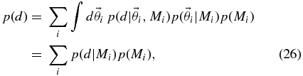
To compare the various models Mi, we are interested in the marginalized posterior probability of Mi:
This is the integral of the posterior over the entire parameter space of model Mi. The marginalized posterior probability of model Mi can be rewritten in terms of the single-model evidence, p(d|Mi) (see Equations (25) and (4)):
Here and throughout, we assume that any of the models in Section 3 are equally likely a priori, so the model priors are equal:
A powerful technique6 for computing p(Mi|d) is the reversible-jump MCMC (Green 1995). Reversible-jump MCMC, discussed in more detail in Appendix B, is a standard MCMC analysis conducted in the super-model. The result of a reversible-jump MCMC is a chain of samples,  , from the super-model parameter space. The integral in Equation (28) can be estimated by counting the number of times that a given model Mi appears in the reversible-jump MCMC chain:
where Ni is the number of MCMC samples that have discrete parameter Mi and N is the total number of samples in the MCMC.
Naively implemented reversible-jump MCMCs can be very inefficient when the posteriors for a model or models are strongly peaked. In this circumstance, a proposed MCMC jump into one of the peaked models is unlikely to land on the peak by chance; since it is rare to propose a jump into the important regions of parameter space of the peaked model in a naive reversible-jump MCMC, the output chain must be very long to ensure that all models have been compared fairly. We describe a new algorithm in Appendix B that produces very efficient jump proposals for a reversible-jump MCMC by exploiting the information about the model posteriors we have from the single-model MCMC samples. (See also Farr & Mandel 2011.) With this algorithm, reasonable chain lengths can fairly compare all the models under consideration. We have used this algorithm to perform 10-way reversible-jump MCMCs to calculate the relative evidence for both the parametric and non-parametric models in this study. These results appear in Section 4.
4. RESULTS
In this section, we discuss the results of our MCMC analysis of the posterior distributions of parameters for the models in Sections 3.3 and 3.4. We also discuss model selection results. The results in Section 4.1 apply to the low-mass sample of systems, while those of Section 4.2 apply to the combined sample of systems.
4.1. Low-mass Systems
Table 2 gives quantiles of the marginalized parameter distributions of the parametric models implied by the low-mass data. Table 3 gives the quantiles of the histogram bin boundaries in the non-parametric analysis implied by the low-mass data.
Table 2. Quantiles of the Marginalized Distribution for Each of the Parameters in the Models Discussed in Section 3.3 Implied by the Low-mass Data
| Model | Parameter | 5% | 15% | 50% | 85% | 95% |
|---|---|---|---|---|---|---|
| Power law (Equation (7)) | Mmin | 1.2786 | 4.1831 | 6.1001 | 6.5011 | 6.6250 |
| Mmax | 8.5578 | 8.9214 | 23.3274 | 36.0002 | 38.8113 | |
| α | −12.4191 | −10.1894 | −6.3861 | 2.8476 | 5.6954 | |
| Exponential (Equation (11)) | Mmin | 5.0185 | 5.4439 | 6.0313 | 6.3785 | 6.5316 |
| M0 | 0.7796 | 0.9971 | 1.5516 | 2.4635 | 3.2518 | |
| Gaussian (Equation (13)) | μ | 6.6349 | 6.9130 | 7.3475 | 7.7845 | 8.0798 |
| σ | 0.7478 | 0.9050 | 1.2500 | 1.7335 | 2.1134 | |
| Two Gaussian (Equation (15)) | μ1 | 5.4506 | 6.3877 | 7.1514 | 7.6728 | 7.9803 |
| μ2 | 7.2355 | 7.7387 | 12.3986 | 25.2456 | 31.4216 | |
| σ1 | 0.3758 | 0.7626 | 1.2104 | 1.7981 | 2.3065 | |
| σ2 | 0.2048 | 0.6421 | 1.9182 | 5.2757 | 7.2625 | |
| α | 0.0983 | 0.3526 | 0.8871 | 0.9792 | 0.9936 | |
| Log normal (Equation (17)) | 〈M〉 | 6.7619 | 7.0122 | 7.4336 | 7.9159 | 8.2942 |
| σM | 0.7292 | 0.8920 | 1.2704 | 1.8695 | 2.4069 | |
Notes. We indicate the 5%, 15%, 50% (median), 85%, and 95% quantiles. The marginalized distribution can be misleading when there are strong correlations between variables. For example, while the marginalized distributions for the power-law parameters are quite broad, the distribution of mass distributions implied by the power-law MCMC samples is similar to the other models. This occurs in spite of the broad marginalized distributions because of the correlations between the slope and limits of the power law discussed in Section 3.3.1.
Download table as: ASCIITypeset image
Table 3. The 5%, 15%, 50% (Median), 85%, and 95% Quantiles for the Bin Boundaries in the One-through Five-bin Histogram Models Discussed in Section 3.4
| Bins | Boundary | 5% | 15% | 50% | 85% | 95% |
|---|---|---|---|---|---|---|
| 1 | w0 | 3.94488 | 4.55603 | 5.43333 | 6.02557 | 6.29749 |
| w1 | 8.50844 | 8.69262 | 9.11784 | 9.83477 | 10.5128 | |
| 2 | w0 | 3.3426 | 4.2047 | 5.39132 | 6.18413 | 6.47553 |
| w1 | 6.41972 | 6.72605 | 7.43421 | 8.2489 | 8.52885 | |
| w2 | 8.46161 | 8.65077 | 9.12694 | 10.1113 | 11.2595 | |
| 3 | w0 | 2.18176 | 3.54345 | 5.16094 | 6.16473 | 6.44697 |
| w1 | 5.68876 | 6.14223 | 6.68829 | 7.38725 | 8.04235 | |
| w2 | 6.8297 | 7.22718 | 8.1451 | 8.7512 | 9.27296 | |
| w3 | 8.44307 | 8.67362 | 9.25718 | 12.1688 | 21.92 | |
| 4 | w0 | 1.32131 | 2.7934 | 4.66156 | 5.78459 | 6.17946 |
| w1 | 5.20112 | 5.77331 | 6.42501 | 6.98427 | 7.44584 | |
| w2 | 6.41805 | 6.73535 | 7.43826 | 8.32958 | 8.64212 | |
| w3 | 7.40302 | 7.95608 | 8.58976 | 9.33897 | 10.3992 | |
| w4 | 8.56724 | 8.8059 | 10.2451 | 24.3573 | 34.2423 | |
| 5 | w0 | 0.9392 | 2.28789 | 4.33389 | 5.7012 | 6.21166 |
| w1 | 4.69778 | 5.44302 | 6.26575 | 6.76407 | 7.14427 | |
| w2 | 6.1388 | 6.47155 | 7.00606 | 7.97325 | 8.38259 | |
| w3 | 6.82058 | 7.28677 | 8.22514 | 8.81555 | 9.41012 | |
| w4 | 8.02335 | 8.36993 | 8.94879 | 11.3206 | 17.3349 | |
| w5 | 8.7112 | 9.25208 | 16.2059 | 31.897 | 37.2738 | |
Download table as: ASCIITypeset image
Recall that each MCMC sample in our analysis gives the parameters for a model of the black hole mass distribution. The chain of samples of parameters for a particular model gives us a distribution of black hole mass distributions. Figure 3 gives a sense of the shape and range of the distributions of black hole mass distributions that result from our MCMC analysis. In Figure 3, we plot the median, 10%, and 90% values of the black hole mass distributions that result from the MCMC chains. Because the choice of parameters that gives, for example, the median distribution value at one mass need not give the median distribution at another mass, these curves do not necessarily look like the underlying model for the mass distribution. For the same reason, they are not necessarily normalized.

Figure 3. Median (solid line), 10% (lower dashed line), and 90% (upper dashed line) values of the black hole mass distribution, p(M|θ), at various masses implied by the posterior p(θ|d) for the models discussed in Sections 3.3 and 3.4. These distributions use only the 15 low-mass observations in Table 1 (the combined sample is analyzed in Section 4.2). Note that these "distributions of distributions" are not necessarily normalized, and need not be shaped like the underlying model distributions.
Download figure:
Standard image High-resolution image4.1.1. Power Law
In Figure 4, we display a histogram of the resulting samples in each of the parameters Mmin, Mmax, and α for the power-law model (see Equation (7)); this represents the one-dimensional "marginalized" distribution
and similarly for Mmin and Mmax.

Figure 4. Histograms of the marginalized distribution for the three parameters Mmin (top, left), Mmax (top, right), and α (bottom) from the power-law model. The marginalized distribution for α is broad, with −11.8 < α < 6.8 enclosing 90% of the probability. We have p(α < 0) = 0.6; the median value is α = −3.35. The broad distribution for α (and the other parameters) is due to correlations between the parameters discussed in the main text; see Figure 5.
Download figure:
Standard image High-resolution imageThe marginalized distribution for α is broad, with

enclosing 90% of the probability (excluding 5% on each side). We have p(α < 0) = 0.6. The median value is α = −3.35. The broadness of the marginalized distribution for α comes from the need to match the relatively narrow range in mass of the low-mass systems. When α is negative, the resulting mass distribution slopes down; Mmin is constrained to be near the lowest mass of the observed black holes, while Mmax is essentially irrelevant. Conversely, when α is positive and the mass distribution slopes up, Mmax must be close to the largest mass observed, while Mmin is essentially irrelevant. Figure 5 illustrates this effect, showing the correlations between α and Mmin and α and Mmax. When we include the high-mass systems in the analysis, the long tail will eliminate this effect by bringing both Mmin and Mmax into play for all values of α.
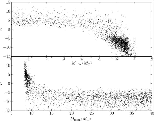
Figure 5. MCMC samples in the Mmin, α (top) and Mmax, α (bottom) planes for the power-law model discussed in Section 3.3.1. The correlations between α and the power-law bounds discussed in the text are apparent: when α is positive, the mass distribution slopes upward and Mmax is constrained to be near the maximum observed mass while Mmin is unconstrained. When α is negative, the mass distribution slopes down and Mmin is constrained to be near the lowest mass observed, while Mmax is unconstrained.
Download figure:
Standard image High-resolution image4.1.2. Decaying Exponential
Figure 6 displays the marginalized posterior distribution for the scale mass of the exponential, M0, and the cutoff mass, Mmin (see Equation 11). The median scale mass is M0 = 1.55, and 0.78 ⩽ M0 ⩽ 3.25 with 90% confidence. This model was one of those considered by Ozel et al. (2010), whose results (M0 ∼ 1.5 and Mmin ∼ 6.5) are broadly consistent with ours. Figure 7 displays the MCMC samples in the Mmin, M0 plane for this model. There is a small correlation between smaller Mmin and larger M0, which is driven by the need to widen the distribution to encompass the peak of the mass measurements in Figure 1 when the minimum mass is smaller.
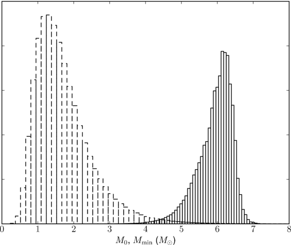
Figure 6. Distribution of scale masses, M0 (dashed histogram), and minimum masses, Mmin (solid histogram), both measured in units of a solar mass for the exponential underlying mass distribution defined in Equation (11). The median scale mass is M0 = 1.55, and 0.78 ⩽ M0 ⩽ 3.25 with 90% confidence.
Download figure:
Standard image High-resolution image
Figure 7. MCMC samples in the Mmin, M0 plane for the decaying exponential underlying mass distribution model. The slight correlation between smaller Mmin and larger M0 is driven by the need to widen the mass distribution to encompass the peak of the measurements in Figure 1 when the minimum mass decreases.
Download figure:
Standard image High-resolution image4.1.3. Gaussian
Figure 8 shows the resulting marginalized distributions for the parameters μ and σ. We constrain the peak of the Gaussian between 6.63 ⩽ μ ⩽ 8.08 with 90% confidence. This model also appeared in Ozel et al. (2010); they found μ ∼ 7.8 and σ ∼ 1.2, consistent with our results here.
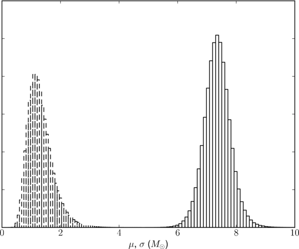
Figure 8. Marginalized posterior distributions for the mean, μ (solid histogram), and standard deviation, σ (dashed histogram), both in solar masses for the Gaussian underlying mass distribution defined in Equation (13). The peak of the Gaussian, μ, is constrained in 6.63 ⩽ μ ⩽ 8.08 with 90% confidence.
Download figure:
Standard image High-resolution image4.1.4. Two Gaussian
Figure 9 shows the marginalized distributions for the two-Gaussian model parameters from our MCMC runs. We find α > 0.8 with 62% probability, clearly favoring the Gaussian with smaller mean. The distributions for μ1 and σ1 are similar to those of the single Gaussian displayed in Figure 8, indicating that this Gaussian is centered around the peaks of the low-mass distributions. The second Gaussian's parameter distributions are much broader. The second Gaussian appears to be sampling the tail of the mass samples. In spite of the extra degrees of freedom in this model, we find that this model is strongly disfavored relative to the single-Gaussian model for this data set:  (see Sections 3.5 and 4.1.7 for discussion).
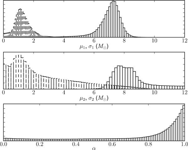
Figure 9. Marginal distributions for the five parameters of the two-Gaussian model. The top panel is μ1 (solid histogram) and σ1 (dashed histogram), the middle panel is μ2 (solid histogram) and σ2 (dashed histogram), and the bottom panel is α. We have α > 0.8 with 62% probability, favoring the first of the two Gaussians. The distributions for μ1 and σ1 are similar to those of the single-Gaussian model displayed in Figure 8; the second Gaussian's parameter distributions are much broader (recall that we constrain μ2 > μ1). The second Gaussian is attempting to fit the tail of the mass samples. The extra degrees of freedom in the distribution from the second Gaussian do not provide enough extra fitting power to compensate for the increase in parameter space, however: the two-Gaussian model is disfavored relative to the single Gaussian by a factor of 4.7 on this data set (see Sections 3.5 and 4.1.7 for discussion).
Download figure:
Standard image High-resolution image4.1.5. Log Normal
The marginal distributions for 〈M〉 and σM appear in Figure 10. The distributions are similar to those for μ and σ from the Gaussian model in Section 3.3.3.
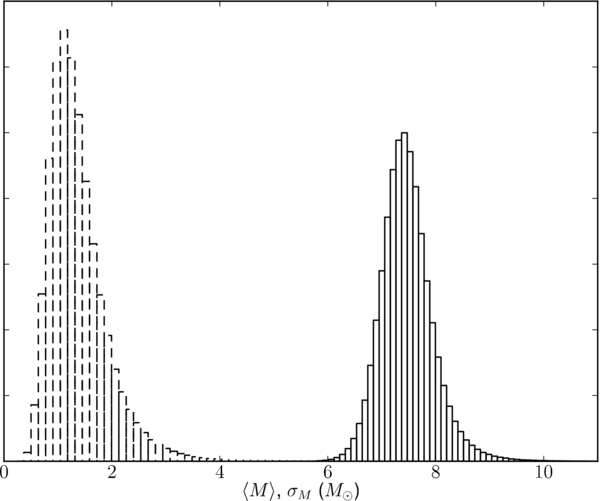
Figure 10. Marginalized distributions of the mean mass, 〈M〉 (solid histogram), and standard deviation of the mass, σM (dashed histogram), for the log-normal model in Section 3.3.4. The distributions are similar to the distributions of μ and σ in the Gaussian model of Section 3.3.3.
Download figure:
Standard image High-resolution image4.1.6. Histogram Models
The median values of the histogram mass distributions that result from the MCMC samples of the posterior distribution for the wi parameters for one-, two-, three-, four-, and five-bin histogram models are shown in Figure 3. Table 3 gives quantiles of the marginalized bin boundary distributions for the histogram models.
As the number of bins increases, the models are better able to capture features of the mass distribution, but we find that the one-bin histogram is the most probable of the histogram models for the low-mass data (see Section 4.1.7 for discussion). This occurs because the extra fitting power does not sufficiently improve the fit to compensate for the vastly larger parameter space of the models with more bins.
4.1.7. Model Selection for the Low-mass Sample
We have performed a suite of 500 independent reversible-jump MCMCs jumping between all the models (both parametric and non-parametric) described in Section 3 using the single-model MCMC samples to construct an efficient jump proposal for each model as described above (see Appendix B). The numbers of counts in each model are consistent across the MCMCs in the suite; Figure 11 displays the average probability for each model across the suite, along with the 1σ errors on the average inferred from the standard deviation of the model counts across the suite. Table 4 gives the numerical values of the average probability for each model across the suite of MCMCs.
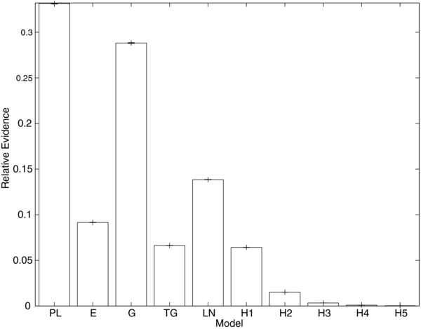
Figure 11. Relative probability of the models discussed in Section 3 as computed using the reversible-jump MCMC with the efficient jump proposal algorithm described in Appedix B. (See also Table 4.) In increasing order along the x-axis, the models are the power law of Section 3.3.1 (PL), the decaying exponential of Section 3.3.2 (E), the single Gaussian of Section 3.3.3 (G), the double Gaussian of Section 3.3.3 (TG), and the one-, two-, three-, four-, and five-bin histogram models of Section 3.4 (H1, H2, H3, H4, H5, respectively). The average of 500 independent reversible-jump MCMCs is plotted, along with the 1σ error on the average inferred from the standard deviation of the probability from the individual MCMCs. As discussed in the text, the power-law and Gaussian models are the most favored.
Download figure:
Standard image High-resolution imageTable 4. Relative Probabilities of the Various Models from Section 3 Implied by the Low-mass Data
| Model | Relative Evidence |
|---|---|
| Power law (Section 3.3.1) | 0.331488 |
| Gaussian (Section 3.3.3) | 0.288129 |
| Log normal (Section 3.3.4) | 0.138435 |
| Exponential (Section 3.3.2) | 0.0916218 |
| Two Gaussian (Section 3.3.3) | 0.0662577 |
| Histogram (1 Bin, Section 3.4) | 0.0641941 |
| Histogram (2 Bin, Section 3.4) | 0.015184 |
| Histogram (3 Bin, Section 3.4) | 0.00332933 |
| Histogram (4 Bin, Section 3.4) | 0.000999976 |
| Histogram (5 Bin, Section 3.4) | 0.0003614 |
Notes. These probabilities have been computed from reversible-jump MCMC samples using the efficient jump proposal algorithm in Appendix B. (See also Figure 11.)
Download table as: ASCIITypeset image
The most favored model is the power law from Section 3.3.1, followed by the Gaussian model from Section 3.3.3. Interestingly, the theoretical curve from Fryer & Kalogera (2001; the exponential model of Section 3.3.2) places fourth in the ranking of evidence.
Though the model probabilities presented in this section have small statistical error, they are subject to large "systematic" error. The source of this error is both the particular choice of model prior (uniform across models) and the choice of priors on the parameters within each model used for this work. For example, the theoretically preferred exponential model (Section 3.3.2) is only a factor of ∼3 away from the power-law model (Section 3.3.1), which does not have theoretical support. Is such support worth a factor of three in the model prior? Alternately, we may say we know (in advance of any mass measurements) that black holes must exist with mass ≲ 10 M☉; then we could, for example, impose a prior on the minimum mass in the exponential model (Mmin) that is uniform between 0 and 10 M☉, which would reduce the prior volume available for the model by a factor of four without significantly reducing the posterior support for the model. This has the same effect as increasing the model prior by a factor of four, which would move this model from fourth to first place. Of course, we would then have to modify the prior support for the other models to take into account the restriction that there must be black holes with M ≲ 10 M☉... Linder & Miquel (2008) discuss these issues in the context of cosmological model selection, concluding with a warning against overreliance on model selection probabilities.
Nevertheless, we believe that our model comparison is reasonably fair (see the discussion of priors in Section 3.2). It seems safe to conclude that "single-peaked" models (the power law and Gaussian) are preferred over "extended" models (the exponential or log normal), or those with "structure" (the many-bin histograms or two-Gaussian model). Previous studies have also supported the "single, narrow peak" mass distribution (Bailyn et al. 1998; Ozel et al. 2010). In this light, poor performance of the single-bin histogram is surprising.
4.2. Combined Sample
This section repeats the analysis of the models from Section 3, but including the high-mass, wind-fed systems from Table 1 (see also Figure 2) in the sample. Figure 12 displays bounds on the value of the underlying mass distribution for the various models in Section 3 applied to this data set; compare to Figure 3. The inclusion of the high-mass, wind-fed systems tends to widen the distribution toward the high-mass end and, in models that allow it, produces a second, high-mass peak in addition to the one in Figure 3.

Figure 12. Median (solid line), 10% (lower dashed line), and 90% (upper dashed line) values of the black hole mass distribution, p(M|θ), at various masses implied by the posterior p(θ|d) for the models discussed in Sections 3.3 and 3.4. These distributions use the combined sample of 20 observations in Table 1, including the high-mass, wind-fed systems. Note that these "distributions of distributions" are not necessarily normalized, and need not be "shaped" like the underlying model distributions. Compare to Figure 3, which includes only the low-mass systems in the analysis. Including the high-mass systems tends to widen the distribution toward the high-mass end and, in models that allow it, to produce a second, high-mass peak in addition to the one in Figure 3.
Download figure:
Standard image High-resolution image4.2.1. Power Law
Figure 13 presents the marginalized distribution for the three power-law parameters Mmin, Mmax, and α (Section 3.3.1) from an analysis including the high-mass systems. The distribution for Mmax is quite broad because the best-fit power laws slope downward (α < 0), making this parameter less relevant. The range −5.05 ⩽ α ⩽ −1.77 encloses 90% of the probability; the median value of α is −3.23. The presence of the high-mass samples in the analysis produces a distinctive tail, eliminating the correlations discussed in Section 3.3.1 and displayed in Figure 5 for the low-mass subset of the observations.
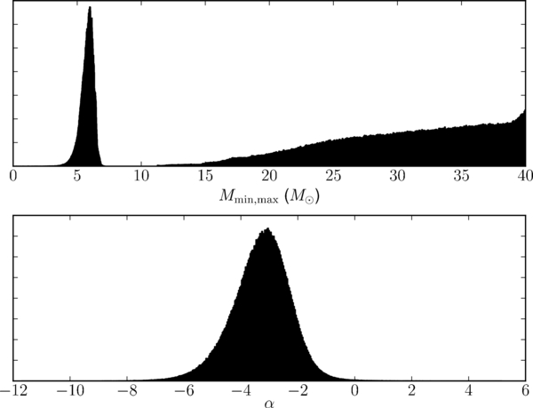
Figure 13. Histograms of the marginalized distribution for the three parameters Mmin (top, left), Mmax (top, right), and α (bottom) from the power-law model including the high-mass samples in the MCMC. The distribution for Mmax is quite broad because the best-fit power laws slope downward (α < 0), making this parameter less relevant. The range −5.05 ⩽ α ⩽ −1.77 encloses 90% of the probability; the median value of α is −3.23. The presence of the high-mass samples in the analysis produces a distinctive tail, eliminating the correlations discussed in Section 3.3.1 and displayed in Figure 5 for the low-mass subset of the observations.
Download figure:
Standard image High-resolution image4.2.2. Decaying Exponential
Figure 14 displays the marginalized distributions for the exponential parameters Mmin and M0 (Section 3.3.2) from an analysis including the high-mass systems. The distribution for the scale mass, M0, has moved to higher masses relative to Figure 6 to fit the tail of the mass distribution; the distribution for Mmin is less affected, though it has broadened somewhat toward low masses.
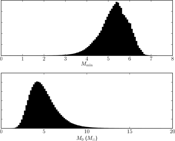
Figure 14. Marginalized distributions for the exponential parameters Mmin (top) and M0 (bottom) defined in Section 3.3.2 from an analysis including the high-mass systems. The distribution for the scale mass, M0, has moved to higher masses relative to Figure 6 to fit the tail of the mass distribution; we now have 2.8292 ⩽ M0 ⩽ 7.9298 with 90% confidence, with median 4.7003. The distribution for Mmin is less affected, though it has broadened somewhat toward low masses.
Download figure:
Standard image High-resolution image4.2.3. Gaussian
Figure 15 displays the marginalized distributions for the Gaussian parameters (Section 3.3.3) when the high-mass objects are included in the mass distribution. The mean mass, μ, and the mass standard deviation, σ, are both increased relative to Figure 8 to account for the broader distribution and high-mass tail.

Figure 15. Marginalized distributions for the Gaussian parameters when the high-mass objects are included in the mass distribution. The mean mass, μ (solid histogram), and the mass standard deviation, σ (dashed histogram), are both increased relative to Figure 8 to account for the broader distribution and high-mass tail. The peak of the underlying mass distribution lies in the range 7.8660 ⩽ μ ⩽ 10.9836 with 90% confidence; the median value is 9.2012.
Download figure:
Standard image High-resolution image4.2.4. Two Gaussian
The analysis of the two-Gaussian model shows the largest change when the high-mass samples are included. Figure 16 shows the marginalized distributions for the two-Gaussian parameters (Section 3.3.3) when the high-mass samples are included in the analysis. In stark contrast to Figure 9, there are two well-defined, separated peaks; the low-mass peak reproduces the results from the low-mass samples, while the high-mass peak (13.5534 ⩽ μ2 ⩽ 27.9481 with 90% confidence; median 20.3839) matches the new high-mass samples. The peak in α near 0.8 is consistent with approximately four-fifths the total probability being concentrated in the 15 low-mass samples.

Figure 16. Marginalized distributions for the two-Gaussian parameters (Section 3.3.3) when the high-mass samples are included in the analysis. The means (μ1 and μ2) are represented by the solid histograms; the standard deviations (σ1 and σ2) are represented by the dashed histograms. In stark contrast to Figure 9, there are two well-defined, separated peaks; the low-mass peak reproduces the results from the low-mass samples, while the high-mass peak (13.5534 ⩽ μ2 ⩽ 27.9481 with 90% confidence; median 20.3839) matches the new high-mass samples. The peak in α near 0.8 is consistent with approximately 15 out of 20 samples belonging to the low-mass peak.
Download figure:
Standard image High-resolution image4.2.5. Log Normal
The marginalized distributions for the log-normal parameters (Section 3.3.4) when the high-mass samples are included in the analysis are displayed in Figure 17. The changes when the high-mass samples are included (compare to Figure 10) are similar to the changes in the Gaussian distribution: the mean mass moves to higher masses and the distribution broadens. Because the log-normal distribution is inherently asymmetric, with a high-mass tail, it does not need to widen as much as the Gaussian distribution did.

Figure 17. Marginalized distributions for the log-normal parameters (Section 3.3.4; 〈M〉 solid, σM dashed) when the high-mass samples are included in the analysis. The changes when the high-mass samples are included (compare to Figure 10) are similar to the changes in the Gaussian distribution: the mean mass moves to higher masses, and the distribution broadens.
Download figure:
Standard image High-resolution imageThe confidence limits on the parameters for the parametric models of the underlying mass distribution are displayed in Table 5 (compare to Table 2).
Table 5. Quantiles of the Marginalized Distribution for Each of the Parameters in the Models Discussed in Section 3.3 when the High-mass Samples are Included in the Analysis (Compare to Table 2)
| Model | Parameter | 5% | 15% | 50% | 85% | 95% |
|---|---|---|---|---|---|---|
| Power law (Equation (7)) | Mmin | 4.87141 | 5.29031 | 5.85019 | 6.26118 | 6.45674 |
| Mmax | 19.1097 | 23.4242 | 31.5726 | 37.7519 | 39.3369 | |
| α | −5.04879 | −4.30368 | −3.23404 | −2.31365 | −1.77137 | |
| Exponential (Equation (11)) | Mmin | 4.0865 | 4.60236 | 5.32683 | 5.94097 | 6.22952 |
| M0 | 2.82924 | 3.41139 | 4.70034 | 6.52214 | 7.92979 | |
| Gaussian (Equation (13)) | μ | 7.86599 | 8.33118 | 9.20116 | 10.2493 | 10.9836 |
| σ | 2.23643 | 2.58899 | 3.33545 | 4.17886 | 4.67881 | |
| Two Gaussian (Equation (15)) | μ1 | 6.741 | 7.02724 | 7.48174 | 8.0139 | 8.46626 |
| μ2 | 13.5534 | 16.202 | 20.3839 | 24.9259 | 27.9481 | |
| σ1 | 0.742824 | 0.913941 | 1.31244 | 1.94862 | 2.50238 | |
| σ2 | 0.511159 | 1.5025 | 4.39824 | 7.04612 | 8.25905 | |
| α | 0.575692 | 0.670978 | 0.798227 | 0.891522 | 0.932143 | |
| Log normal (Equation (17)) | 〈M〉 | 8.00086 | 8.51192 | 9.6264 | 11.1851 | 12.3986 |
| σM | 2.19262 | 2.8137 | 4.16742 | 6.25101 | 8.11839 | |
Note. We indicate the 5%, 15%, 50% (median), 85%, and 95% quantiles.
Download table as: ASCIITypeset image
4.2.6. Histogram Models
The non-parametric (histogram; see Section 3.4) models also show evidence of a long tail from the inclusion of the high-mass samples. Table 6 displays confidence limits on the histogram parameters for the analysis including the high-mass systems; compare to Table 3.
Table 6. The 5%, 15%, 50% (Median), 85%, and 95% Quantiles for the Bin Boundaries in the One-through Five-bin Histogram Models Discussed in Section 3.4 in an Analysis Including the High-mass, Wind-fed Systems
| Bins | Boundary | 5% | 15% | 50% | 85% | 95% |
|---|---|---|---|---|---|---|
| 1 | w0 | 2.22294 | 3.12695 | 4.2456 | 5.15132 | 5.58265 |
| w1 | 15.93 | 16.2535 | 17.7836 | 20.5449 | 22.5836 | |
| 2 | w0 | 3.87202 | 4.49983 | 5.41234 | 6.08334 | 6.35933 |
| w1 | 7.22163 | 8.25079 | 8.93669 | 9.71551 | 10.4287 | |
| w2 | 18.4762 | 19.9798 | 24.941 | 32.5972 | 36.8615 | |
| 3 | w0 | 3.39289 | 4.24509 | 5.41694 | 6.15087 | 6.42822 |
| w1 | 6.41849 | 6.71984 | 7.47263 | 8.2942 | 8.61785 | |
| w2 | 8.41449 | 8.64664 | 9.17056 | 10.4075 | 12.2718 | |
| w3 | 18.5705 | 21.0481 | 27.1494 | 34.7753 | 38.0652 | |
| 4 | w0 | 2.42094 | 3.69875 | 5.2596 | 6.25449 | 6.54316 |
| w1 | 5.83725 | 6.2836 | 6.84987 | 7.8033 | 8.27706 | |
| w2 | 6.94919 | 7.43628 | 8.38531 | 9.13401 | 9.91845 | |
| w3 | 8.50371 | 8.75188 | 9.86694 | 17.1848 | 22.1086 | |
| w4 | 18.5823 | 21.4628 | 28.367 | 35.8118 | 38.5278 | |
| 5 | w0 | 1.73691 | 3.19184 | 4.89769 | 5.9547 | 6.35522 |
| w1 | 5.46124 | 5.95881 | 6.59431 | 7.26795 | 7.91821 | |
| w2 | 6.63468 | 6.9804 | 7.93239 | 8.60918 | 9.06926 | |
| w3 | 7.89654 | 8.35634 | 8.91766 | 10.6568 | 13.9644 | |
| w4 | 8.74064 | 9.42672 | 15.8004 | 22.7101 | 27.6399 | |
| w5 | 20.0202 | 22.9065 | 29.6307 | 36.6606 | 38.8573 | |
Note. The tails evident in Figure 12 are apparent here as well; compare to Table 3.
Download table as: ASCIITypeset image
4.2.7. Model Selection for the Combined Sample
Repeating the model selection analysis discussed in Section 4.1.7 for the sample including the high-mass systems, we find that the model probabilities have changed with the inclusion of the extra five systems. As before, we assume for this analysis that the model priors are equal.
Reversible-jump MCMC calculations of the model probabilities are displayed in Figure 18; compare to Figure 11. The relative model probabilities are given in Table 7. The exponential model is the most favored model for the combined sample, with the two-Gaussian model the second-most favored. The ranking of models differs significantly from the low-mass samples. The improvement of the exponential model relative to the low-mass analysis is encouraging for theoretical calculations that attempt to model the entire population of X-ray binaries with this mass model. Note also that the increasing structure of the mass distribution favors histogram models with three bins over those with fewer bins.
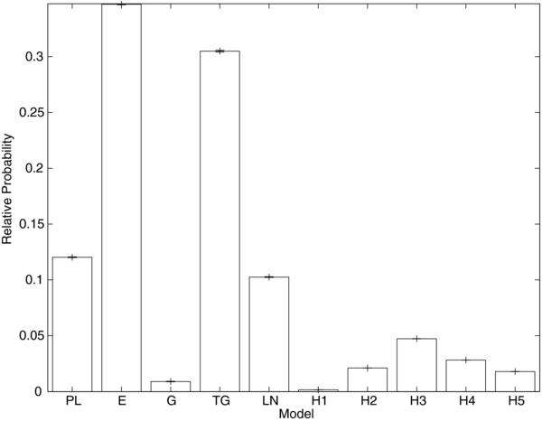
Figure 18. Relative probability of the models discussed in Section 3 as computed using the reversible-jump MCMC with the efficient jump proposal algorithm described in Appendix B, applied to all 20 systems in Table 1 (i.e., including the high-mass systems). (See also Table 7.) In increasing order along the x-axis, the models are the power law of Section 3.3.1 (PL), the decaying exponential of Section 3.3.2 (E), the single Gaussian of Section 3.3.3 (G), the double Gaussian of Section 3.3.3 (TG), and the one-, two-, three-, four-, and five-bin histogram models of Section 3.4 (H1, H2, H3, H4, H5, respectively). The average of 500 independent reversible-jump MCMCs is plotted, along with the 1σ error on the average inferred from the standard deviation of the probability from the individual MCMCs. Compare to Figure 11.
Download figure:
Standard image High-resolution imageTable 7. Relative Probabilities of the Various Models from Section 3 Implied by the Combined Sample of Systems
| Model | Relative Evidence |
|---|---|
| Exponential (Section 3.3.2) | 0.346944 |
| Two Gaussian (Section 3.3.3) | 0.304923 |
| Power law (Section 3.3.1) | 0.120313 |
| Log normal (Section 3.3.4) | 0.102536 |
| Histogram (3 Bin, Section 3.4) | 0.0473464 |
| Histogram (4 Bin, Section 3.4) | 0.0282086 |
| Histogram (2 Bin, Section 3.4) | 0.0210994 |
| Histogram (5 Bin, Section 3.4) | 0.0179703 |
| Gaussian (Section 3.3.3) | 0.00901719 |
| Histogram (1 Bin, Section 3.4) | 0.00164214 |
Note. These probabilities have been computed from reversible-jump MCMC samples using the efficient jump proposal algorithm in Appendix B. (See also Figure 18.)
Download table as: ASCIITypeset image
5. THE MINIMUM BLACK HOLE MASS
It is interesting to use our models for the underlying black hole mass distribution in X-ray binaries to place constraints on the minimum black hole mass implied by the present sample. Bailyn et al. (1998) addressed this question in the context of a "mass gap" between the most massive neutron stars and the least massive black holes. The more recent study of Ozel et al. (2010) also looked for a mass gap using a subset of the models and systems presented here. Both works found that the minimum black hole mass is significantly above the maximum neutron star mass (Kalogera & Baym 1996) of ∼3 M☉ (though Ozel et al. 2010 only state their evidence for a gap in terms of the maximum-posterior parameters and not the full extent of their distributions).
The distributions of the minimum black hole mass from the analysis of the low-mass samples are displayed in Figure 19. The minimum black hole mass is defined as the 1% mass quantile,  , of the black hole mass distribution (i.e., the mass lying below 99% of the mass distribution). (A quantile-based definition is necessary in the case of those distributions that do not have a hard cutoff mass; even for those that do, like the power-law model, it can be useful to define a "soft" cutoff in the event that the lower-mass hard cutoff becomes an irrelevant parameter as discussed in Section 3.3.1.) For each mass distribution parameter sample from our MCMC, we can calculate the distribution's minimum black hole mass; the collection of these minimum black hole masses approximates the distribution of minimum black hole masses implied by the data in the context of that distribution. Figure 19 plots histograms of the minimum black hole mass samples.

Figure 19. Distributions for the minimum black hole mass,  , calculated from the MCMC samples for the models in Section 3 applied to the low-mass systems. For the most favored models, the power law and Gaussian, the 90% confidence limit on the minimum black hole mass is 4.3 M☉ and 2.9 M☉, respectively. In all plots, we indicate the 90% confidence bound (i.e., the 10% quantile) on the minimum black hole mass with a vertical line.
Download figure:
Standard image High-resolution imageWe find that the best-fit model for the low-mass systems (the power law) has  in 90% of the MCMC samples (i.e., at 90% confidence). This is significantly above the maximum theoretically allowed neutron star mass, ∼3 M☉ (e.g., Kalogera & Baym 1996). Hence, we conclude that the low-mass systems show strong evidence of a mass gap.
The distribution of minimum black hole masses for the analysis of the combined sample (i.e., including the high-mass systems) is shown in Figure 20. For the most favored model, the exponential, we find that  with 90% confidence. We therefore conclude that there is strong evidence for a mass gap in the combined sample as well.

Figure 20. Distributions for the minimum black hole mass,  , calculated from the MCMC samples for the models in Section 3 using the combined sample of systems. For the two most favored models, the exponential and two Gaussian, the 90% confidence limit on the minimum black hole mass is 4.5 M☉ and 2.3 M☉, respectively. For every model, we indicate the 90% confidence bound on the minimum black hole mass with a vertical line.
Download figure:
Standard image High-resolution imageTable 8 gives the 10%, 50% (median), and 90% quantiles for the minimum black hole mass implied by the low-mass sample; Table 9 gives the same, but for the combined sample of systems.
Table 8. The 10%, 50% (Median), and 90% Quantiles for the Minimum Black Hole Mass (in Units of M☉) Implied by the Low-mass Sample in the Context of the Various Models for the Black Hole Mass Distribution
| Model | 10% | 50% | 90% |
|---|---|---|---|
| Power law (Section 3.3.1) | 4.3 | 6.1 | 6.6 |
| Gaussian (Section 3.3.3) | 2.9 | 4.4 | 5.5 |
| Log normal (Section 3.3.4) | 3.9 | 4.9 | 5.8 |
| Exponential (Section 3.3.2) | 5.3 | 6.0 | 6.5 |
| Two Gaussian (Section 3.3.3) | 2.4 | 4.2 | 5.5 |
| Histogram (1 Bin, Section 3.4) | 4.4 | 5.5 | 6.2 |
| Histogram (2 Bin, Section 3.4) | 4.0 | 5.4 | 6.3 |
| Histogram (3 Bin, Section 3.4) | 3.2 | 5.2 | 6.3 |
| Histogram (4 Bin, Section 3.4) | 2.4 | 4.7 | 6.0 |
| Histogram (5 Bin, Section 3.4) | 1.9 | 4.4 | 6.0 |
Note. The models are listed in order of preference from model selection (Section 4.1.7, Figure 11, and Table 4).
Download table as: ASCIITypeset image
Table 9. The 10%, 50% (Median), and 90% Quantiles for the Distribution of Minimum Black Hole Masses (in Units of M☉) Implied by the Combined Sample in the Context of the Various Models for the Black Hole Mass Distribution
| Model | 10% | 50% | 90% |
|---|---|---|---|
| Exponential (Section 3.3.2) | 4.5 | 5.4 | 6.1 |
| Two Gaussian (Section 3.3.3) | 2.3 | 4.3 | 5.5 |
| Power law (Section 3.3.1) | 5.1 | 5.9 | 6.4 |
| Histogram (3 Bin, Section 3.4) | 4.0 | 5.5 | 6.3 |
| Histogram (4 Bin, Section 3.4) | 3.4 | 5.3 | 6.4 |
| Histogram (2 Bin, Section 3.4) | 4.4 | 5.5 | 6.2 |
| Histogram (5 Bin, Section 3.4) | 2.8 | 5.0 | 6.2 |
| Gaussian (Section 3.3.3) | −0.64 | 1.4 | 3.4 |
| Histogram (1 Bin, Section 3.4) | 2.9 | 4.4 | 5.5 |
Note. The models are listed in order of preference from model selection (Section 4.2.7, Figure 18, and Table 7).
Download table as: ASCIITypeset image
6. SUMMARY AND CONCLUSION
We have presented a Bayesian analysis of the mass distribution of stellar-mass black holes in X-ray binary systems. We considered separately a sample of 15 low-mass, Roche lobe filling systems and a sample of 20 systems containing the 15 low-mass systems and 5 high-mass, wind-fed X-ray binaries. We used MCMC methods to sample the posterior distributions of the parameters implied by the data for five parametric models and five non-parametric (histogram) models for the mass distribution. For both sets of samples, we used reversible-jump MCMCs (exploiting a new algorithm for efficient jump proposals in such calculations) to perform model selection on the suite of models. The consideration of a broad range of models and the model selection analysis, along with consideration of the full posterior distribution on the minimum black hole mass, significantly expand earlier statistical analyses of black hole mass measurements (Bailyn et al. 1998; Ozel et al. 2010).
For the low-mass systems, we found the limits on model parameters in Tables 2 and 3. The relative model probabilities from the model selection are given in Table 4. The most favored model for the low-mass systems is a power law. The equivalent limits on the model parameters for the combined systems are given in Tables 5 and 6. Unlike the low-mass systems, the most favored model for the combined sample is the exponential model. This difference indicates that the low-mass subsample is not consistent with being drawn from the distribution of the combined population.
We found strong evidence for a mass gap between the most massive neutron stars and the least massive black holes. For the low-mass systems, the most favored, power-law model gives a black hole mass distribution whose 1% quantile lies above 4.3 M☉ with 90% confidence. For the combined sample of systems, the most favored, exponential model gives a black hole mass distribution whose 1% quantile lies above 4.5 M☉ with 90% confidence. Although the study methodology was different, the existence of a mass gap was pointed out first by Bailyn et al. (1998) and most recently by Ozel et al. (2010) (who did not consider a power-law model, and applied both Gaussian and exponential models to the low-mass systems, where the exponential is strongly disfavored compared to our power-law model).
Theoretical expectations for the black hole mass distribution have been examined in Fryer & Kalogera (2001). They considered results of supernova explosion and fallback simulations (Fryer 1999) applied to single star populations; they also included a heuristic treatment of the possible effects of binary evolution on the black hole mass distribution. It is interesting that we find the most favored model for the combined sample to be an exponential, as discussed by Fryer & Kalogera (2001). On the other hand, we find the most favored model for the low-mass sample to be a power law, with the exponential model strongly disfavored for this sample. In agreement with Bailyn et al. (1998) and Ozel et al. (2010), we too conclude that both the low-mass and combined samples require the presence of a gap between 3 and 4–4.5 M☉.
Fryer (1999) discussed two possible causes of such a gap: (1) a step-like dependence of supernova energy on progenitor mass or (2) selection biases. Current simulations of core collapse in massive stars may shed light on the dependence of supernova energy on progenitor mass. Selection biases can occur because the X-ray binaries with very low mass black holes systems are more likely to be persistently Roche lobe overflowing, preventing dynamical mass measurements. Ozel et al. (2010) conclude that the presence of such biases is not enough to account for the gap, arguing that the number (Equation (26)) of observed persistent X-ray sources not known to be neutron stars is insufficient to populate the 2–5 M☉ region of any black hole mass distribution that rises toward low masses. Population synthesis models incorporating sophisticated treatment of binary evolution and transient behavior (e.g., Fragos et al. 2008, 2009) could help shed light on this possibility.
W.M.F., N.S., and V.K. are supported by NSF grants CAREER AST-0449558 and AST-0908930. A.C., L.K., and C.D.B. are supported by NSF grant NSF/AST-0707627. I.M. acknowledges support from the NSF AAPF under award AST-0901985. Calculations for this work were performed on the Northwestern Fugu cluster, which was partially funded by NSF MRI grant PHY-0619274. We thank Jonathan Gair for helpful discussions.
APPENDIX A: MARKOV CHAIN MONTE CARLO
MCMC methods produce a Markov chain (or sequence) of parameter samples,  , such that a particular parameter set,
  , appears in the sequence with a frequency equal to its probability according to a posterior,
  . A Markov chain has the property that the transition probability from one element to the next,
  , depends only on the value of
  , not on any previous values in the chain.
One way to produce a sequence of MCMC samples is via the following algorithm, first proposed by Metropolis et al. (1953) and used widely in the physical sciences thereafter.
- 1.Begin with the current sample,
 .
. - 2.Propose a new sample,, by drawing randomly from a "jump proposal distribution" with probability . Note that can depend on the current parameters, , and any other "constant" data, but cannot examine the history of the chain beyond the most recent point. This is necessary to preserve the Markovian property of the chain.
- 3.Compute the "acceptance" probability,
- 4.With probability min (1, paccept) "accept" the proposed, setting ; otherwise set .


This algorithm is more likely to accept a proposed jump when it increases the posterior (the first factor in Equation (A1)) and when it is to a location in parameter space from which it is easy to return (the second factor in Equation (A1)); the combination of these influences in Equation (A1) ensures that the equilibrium distribution of the chain is  . As i → ∞ the samples
  are distributed according to
  .
.
In practice the number of samples required before the chain appropriately samples  depends strongly on the jump proposal distribution; proposal distributions that often propose jumps toward or within regions of large
  can be very efficient, while poor proposal distributions can require prohibitively large numbers of samples before convergence.
There is no foolproof test for the convergence of a chain. In this work, we test the convergence of our chains in several ways. The most basic is by comparing the statistics calculated from the entire chain to statistics calculated from only the first half of the chain; when the chain has converged, the two calculations agree. This is a necessary, but not sufficient, condition for convergence.
We also have examined the sample traces from our chains, to see that the chains have densely and randomly sampled parameter space. A representative sample trace from our MCMC for the power-law model applied to the low-mass systems appears in Figure 21. Sample traces from MCMCs with other models are similar.

Figure 21. Parameter sample traces from the MCMC applying the power-law model to the low-mass systems (the parameter histograms for this MCMC appear in Figure 4). For clarity, only every 100th sample point is plotted. The chain is well converged—it samples the regions of posterior support densely and randomly, without any visible trends or sticking points.
Download figure:
Standard image High-resolution imageFinally, for our most quantitative test of convergence we use the gibbsit code to implement the Raftery–Lewis convergence test for our quantile measures (Raftery & Lewis 1992a, 1992b, 1995). The most extreme quantile is the most difficult to determine accurately because—by design—there will be fewer samples in the tail than in the main body of a distribution obtained from an MCMC. Accordingly, we focus on the 90% confidence limit on the minimum black hole mass. For a quantile, q, the Raftery–Lewis test attempts to estimate how many samples from an MCMC are needed to determine q to within ±r at a confidence s. We use r = 0.0125 and s = 0.95. The Raftery–Lewis test approximates the MCMC chain as a two-state Markov chain, the two states being "within the quantile in question" and "outside the quantile in question." The 2 × 2 transition matrix for this two-state Markov chain and the associated uncertainty can be calculated analytically (Raftery & Lewis 1992a, 1992b, 1995), allowing the algorithm to determine the number of sample points required before the quantile of interest is determined sufficiently accurately.
For our chains, in the worst case (the power law on the lower-mass samples, as shown in Figures 4 and 21), we have twice as many samples as the Raftery–Lewis convergence test estimates we need to determine the 90% confidence level on the minimum mass; for all the other chains, we have about 20 times as many samples as the Raftery–Lewis criterion estimates are required. We suspect that the slow convergence of the power-law model on the lower-mass systems is due to the long tails in the mass parameters and the width of the distribution on the power-law exponent. In any case, the Raftery–Lewis test indicates that all our chains are converged sufficiently to determine the 90% quantile to within ∼1%.
We begin the chain at an arbitrary point in parameter space; this is equivalent to taking a finite section of an infinite chain that begins with the chosen point. Every point in parameter space occurs in an infinite chain, and no section of the chain is better than any other, so a sufficiently long, but finite, section of the infinite chain chosen in this manner can be representative of the statistics of the chain as a whole. However, because consecutive samples in a chain are correlated with each other, the beginning of our finite chain has a "memory" of the starting point; we discard enough points at the beginning of the finite chain that we can be confident it does not retain a memory of the arbitrary starting point. The points discarded in this way are commonly called "burn-in" points.
APPENDIX B: REVERSIBLE-JUMP MCMC
The algorithm described here for the reversible-jump MCMC we have used for the model comparison in this work is more fully described in Farr & Mandel (2011). In particular, Farr & Mandel (2011) demonstrate the efficiency gains from the algorithm, and show experimentally that the algorithm indeed provides a consistent reversible-jump MCMC, with the correct relative model probabilities for the case where the Bayes factor between models can be calculated analytically.
Consider the problem of model selection among a set of models, and the "super-model" that encompasses all the models under consideration. The parameter space of the super-model consists of a discrete parameter that identifies the choice of model, Mi, and the continuous parameters appropriate for this model,  . We denote a point in the super-model parameter space by
  ; each such point is a statement that, e.g., "the underlying mass distribution for black holes in the galaxy is a Gaussian, with parameters μ and σ," or "the underlying mass distribution for black holes in the galaxy is a triple-bin histogram with parameters w1, w2, w3, and w4," or... To compare models, we are interested in the quantity (see Equation (27)):
If we perform an MCMC in the super-model parameter space, then we obtain a chain of samples  distributed in parameter space with density
  and we can estimate the integral as
where Ni is the number of samples in the chain lying in the parameter space of model Mi and N is the total number of samples in the chain. The fraction of samples lying in the parameter space of model Mi gives the probability of that model relative to the other models under consideration.
To perform the MCMC in the super-model parameter space, we must propose jumps not only between points in a particular model's parameter space, but also between the parameter spaces of different models. For this MCMC to be efficient, proposed jumps into a model from another should favor regions with large posterior; when the posterior is highly peaked in a small region of parameter space, proposed jumps outside this region are unlikely to be accepted, and the reversible-jump MCMC samples will require a very long chain to properly sample the "super-model" posterior.
We can exploit the information we have from single-model MCMCs to generate efficient jump proposal distributions for our reversible-jump MCMC. We would like to propose jumps that roughly follow the distribution of samples in the single-model MCMCs. We can do this by assigning a neighborhood to each point in the sample using an algorithm we will describe in the following paragraphs; the neighborhoods are non-overlapping, completely cover the region of parameter space with prior support, and contain only one point from the MCMC samples. To propose a jump into model Mi, we choose a point uniformly from that single-model MCMC and then propose a jump drawn uniformly from that point's neighborhood. This is equivalent to drawing from a piecewise-constant approximation to the single-model posterior, where each neighborhood contributes a constant fraction, 1/Ni, to the cumulative jump probability. In regions of high density the neighborhoods are smaller, and the jump probability density is correspondingly higher. Because the neighborhoods cover the entire region of prior support, it is possible for the proposal to propose any point in parameter space with prior support (though points in regions of low single-model posterior are of course unlikely to be proposed).
To assign a neighborhood to each point in a single-model MCMC we use a data structure called a kD-tree. A kD-tree is a binary space-partitioning tree. To construct a kD-tree, we begin with the set of points from a single-model MCMC and a box in parameter space bounding the region of prior support (which must necessarily enclose all the points). The construction proceeds recursively: we choose a dimension7 along which to divide the points, find the median point along that dimension and its nearest neighbor, and divide the box at the midpoint between these two points, producing two sub-boxes. We then partition the points into those to the left (i.e., smaller coordinate along the given dimension) and right of the dividing line, and repeat this procedure for each subset and the corresponding bounding box, until we have only one point in each box. An example of the neighborhoods that result from a two-dimensional kD-tree constructed around a Gaussian point distribution appears in Figure 22.

Figure 22. Neighborhoods constructed from a two-dimensional kD-tree built from a sample of points with a Gaussian density distribution. Each line on the figure corresponds to a sub-dividing box boundary drawn between the median of a subset of the sample points and its nearest neighbor. The peak of the Gaussian lies in the center of the figure; here the point density is highest and the neighborhoods are smallest. Near the edges the density is lower, and the neighborhoods correspondingly larger. The tree adapts itself to the local density of points. If these were single-model MCMC samples, the corresponding jump proposal would first select one of the boxes uniformly at random, and then choose a point uniformly within the box to propose. Since there are many more boxes near the center (each box corresponds to one point), and these boxes are smaller, the proposal will tend to concentrate its points there, approximately tracking the distribution of single-model MCMC samples.
Download figure:
Standard image High-resolution image
Construction of a kD-tree is an  operation, where N is the number of points in the tree. The median finding is
  , where n is the number of points from which the median is to be obtained. At level i in the tree, there are 2i subsets of points, each of length
  , so the total cost of the 2i median calculations is
  at each level. There are
  levels in the tree, yielding a total construction cost for the tree of
  .
.
To find the neighborhood of a point using the tree, we begin at the root of the tree, and examine the two sub-boxes at the next level down. The point will be in one of them; following that branch, we have again two sub-boxes, one of which contains the point; following that branch... Eventually, the search terminates at a leaf of the tree, containing the point in question. The box at the leaf defines the neighborhood of the point in the jump proposal algorithm described above. The total cost for this operation is proportional to the number of levels in the tree, which is  .
.
In addition to the validation tests in Farr & Mandel (2011), we have validated our interpolation method with the following test. We imagine that we have a data set that can be fit by two models: an "egg-crate" model with likelihood
and a single-Gaussian model with likelihood
where the number of dimensions in each parameter space is N = 5, and we choose 2n = 10 peaks along each dimension for the egg-crate model. We restrict the parameter space to ![$\vec{\theta }\in [0,1]^N$](https://content.cld.iop.org/journals/0004-637X/741/2/103/revision1/apj403391ieqn76.gif) , and choose a uniform prior on
, and choose a uniform prior on  within that region. We choose μi = 1/2, and σi = 1/(20i), so the Gaussian peak is well contained within the region of interest, being at least 10σ away from the boundaries of the region. From the point of view of a (reversible-jump) MCMC, the precise data that could produce such unusual likelihoods from two models are irrelevant; the algorithm only cares about the form of the likelihood and prior functions in parameter space. These likelihood functions provide a good test case for our interpolation technique: the egg-crate model has a broad, multi-modal likelihood, while the Gaussian model's likelihood is very concentrated in a small region of parameter space. Particularly for the Gaussian model, a reversible-jump MCMC without interpolation—one that proposes intermodel jumps from the prior, for example—would be extremely inefficient because the region of parameter space with significant posterior support is so small.
Our choice of likelihood and prior implies that the models have equal evidence:
Using individual MCMC parameter samples to construct interpolations of the single-model posterior, and running a 106 sample reversible-jump MCMC, we find
which has an error of 3 × 10⁻³, of the order of  , as would be expected for 1M independent samples from a binomial distribution with p = 0.5. We conclude, as in Farr & Mandel (2011), that our interpolation method leads to accurate and efficient reversible-jump MCMCs.
Footnotes
- 5
A similar analysis of the neutron star mass distribution can be found in Finn (1994).
- 6
We also attempted to compute p(Mi|d) using two other methods: the well-known harmonic-mean estimator and the direct integration methods described in Weinberg (2010). The harmonic mean is known to be very sensitive to outlying points in the MCMC in general, and we found this to be true in our specific application. The statistical properties of the direct integration algorithm from Weinberg (2010) are less certain, but we found that it was quite noisy in our application compared to the reversible-jump MCMC. Due to the statistical noise in the other two methods, we use the results from our reversible-jump MCMC analysis for model selection.
- 7
Our algorithm chooses the dimension along which the numerical extent of the points is largest. Other choices are possible; some algorithms cycle through the dimensions in order, while others choose a random dimension for each subdivision. Our goal by picking the longest dimension is to produce neighborhoods that are "square," at least in the chosen parameterization.